Multi-field coupling dynamic response analysis of pipelines with double corrosion defects under seismic loading in cold regions

Li, Qiao Zhen; Liu, Yang; Wei, Li Xin; Luo, Min

doi:10.21595/jve.2018.19300

Journal of Vibroengineering

Browse Journal

Submit article

Published: 15 August 2018

Check for updates

Multi-field coupling dynamic response analysis of pipelines with double corrosion defects under seismic loading in cold regions

Qiao Zhen Li¹

Yang Liu²

Li Xin Wei³

Min Luo⁴

^{1, 2, 3}School of Petroleum Engineering, Northeast Petroleum University, Daqing, China

⁴College of Mechanical Science and Engineering, Northeast Petroleum University, Daqing, China

Corresponding Author:

Qiao Zhen Li

Cite the article Download PDF

Downloads 1860

WoS Core Citations 1

Abstract

Multi-field coupling system in the paper is composed of the corroded pipelines, fluid, heat preservation layers and frost -heaving soil, and the buried pipelines are inevitable to be affected by earthquakes, but few studies have been done on corroded pipelines in multi-field coupling under seismic loading in cold regions. The paper analyzes the dynamic response of the pipelines under seismic loading. Method by FEM (finite element method), the three-dimensional multi-field coupling mechanics model has been established for analysis, based on a thermal-fluid-solid multi-field coupling analysis theory, considering the actual stress-strain characteristics of the pipeline steel and the frost heaving force of soil. Meanwhile, the influences of fluid pressure, fluid temperature, corrosion defects and seismic waves on the mechanical properties of the pipelines are then discussed. The results show that: the relative corrosion depth, fluid pressure and fluid temperature have obvious influence on the mechanical properties of corroded pipelines; other factors are relatively weak; the properties of corroded pipelines do not change with different seismic loading. For the corroded pipelines in cold regions, the factors which have obvious influence on the mechanical properties of pipelines should be monitored intensely.

1. Introduction

With the increasing demand for oil and gas resources in China, the pipelines in cold regions have found an increasingly wide utilization, which play a more and more important role in the development of national economy. Due to the particularity of the environment in cold regions, the pipelines not only bear the risks of corrosion, mechanical damage, third-party damage, and so on like the pipelines in ordinary regions, but also the risks of thawing, frost heaving, ice jam, exposed pipelines and others [1-3].

At present, the researches on pipelines in cold regions at home and abroad mainly include the stress, strain, displacement of pipelines [4-7], stability analysis [3, 8], wall thickness selection [9] and so on under the action of frost heaving [2]. The numerical simulation method is currently used to study the stress and displacement [10] and the related influence factors for the pipelines under seismic loading [11, 12]. The pipelines in cold regions together with the particular environment compose a multi-field coupling system. Once failures of the system occur, they will cause a series of serious consequences [13]. Additionally, earthquakes often happen in China, and the pipelines in cold regions will inevitably face the risk of earthquakes. However, there is little research about the corroded pipelines in cold regions considering the seismic loading and the multi-field coupling effect.

Aiming at the above problems, FEM (finite element method) is used to analyze the dynamic response of the buried corroded pipelines in cold regions considering the multi-field coupling effect, and the mechanical properties of the pipelines changed with fluid temperature, fluid pressure, corrosion defects and different seismic waves are then discussed. The results can provide an analytical method and a theoretical basis for the integrity evaluation of pipelines in cold regions.

2. Physical model

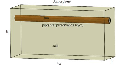
The length of the pipeline selected is 182.8km, the specification of the pipeline is Ø377×6.4 mm, the thickness of heat preservation layer made of rigid polyurethane foam is 40 mm, and the settling depth (from surface to the top of pipeline) is 1.5 m.

The soil itself has a temperature field. From the ground depth ( $H)$ and half of the pipeline horizontal radial $(L / 2)$ , the pipeline has almost no thermal effect on it. The depth ( $H)$ is the constant temperature layer of the soil, and the temperature is $T_{0}^{'}$ ; half of the horizontal radial $(L / 2)$ is considered as adiabatic [14]. Therefore, the object of study can be simplified into a rectangular area according to the thermal effect area, as shown in Fig. 1.

A complex thermal-fluid-solid multi-field coupling model is composed of the corroded pipeline, the fluid in the pipeline, the heat preservation layers and the soil; the fluid-solid coupling model is composed of the corroded pipeline and the fluid in the pipeline; the thermal-solid coupling model is composed of the corroded pipeline, the thermal insulation layer and the soil. The fluid pressure and fluid temperature inside the corroded pipeline are calculated by fluid-solid coupling. The frost heave force and temperature loading outside the corroded pipeline are calculated by thermal-solid coupling. The seismic loading propagation on the pipeline is through the soil.

Fig. 1Three-dimensional physical model

3. Multi-field coupling mathematical model

3.1. Temperature field control equation

The oil in the long-distance pipeline is continuously dissipating heat from the pipeline, so there is an axial temperature loss. In the paper, corroded pipeline, fluid, heat preservation layer and soil are selected as the research object, and the factors which influence the mechanical properties of pipelines with double corrosion defects are mainly analyzed. Considering that the length of pipe in the research is much shorter compared with the length of long-distance pipelines, so it can be approximately considered that there is no temperature loss in the axial direction. The differential equations [15, 16] for heat balance control of temperature field are shown in Eqs. (1-4) respectively.

In the frozen area:

1

ρ_{f} C_{f} \frac{\partial T_{f}}{\partial τ} = \frac{\partial}{\partial x} (λ_{f} \frac{\partial T_{f}}{\partial x}) + \frac{\partial}{\partial y} (λ_{f} \frac{\partial T_{f}}{\partial y}) .

In the thawing area:

2

ρ_{u} C_{u} \frac{\partial T_{u}}{\partial τ} = \frac{\partial}{\partial x} (λ_{u} \frac{\partial T_{u}}{\partial x}) + \frac{\partial}{\partial y} (λ_{u} \frac{\partial T_{u}}{\partial y}) .

Differential equation of unsteady heat conduction for pipeline steel:

3

ρ_{1} C_{1} \frac{\partial T_{1}}{\partial τ} = λ_{1} (\frac{\partial^{2} T_{1}}{\partial r^{2}} + \frac{1}{r} \frac{\partial T_{1}}{\partial r} + \frac{1}{r^{2}} \frac{\partial^{2} T_{1}}{\partial θ^{2}}) .

Differential equation of unsteady heat conduction for heat preservation layer:

4

ρ_{2} C_{2} \frac{\partial T_{2}}{\partial τ} = λ_{2} (\frac{\partial^{2} T_{2}}{\partial r^{2}} + \frac{1}{r} \frac{\partial T_{2}}{\partial r} + \frac{1}{r^{2}} \frac{\partial^{2} T_{2}}{\partial θ^{2}}) .

where $λ_{f}$ , $λ_{u}$ , $λ_{1}$ , $λ_{2}$ are the thermal conductivity of frozen soil , thawing soil, pipeline and heat preservation layer respectively; $ρ_{f}$ , $ρ_{u}$ , $ρ_{1}$ , $ρ_{2}$ are the density of frozen soil , thawing soil, pipeline and heat preservation layer respectively; $C_{f}$ , $C_{u}$ , $C_{1}$ , $C_{2}$ are the heat capacity of frozen soil, thawing soil, pipeline and heat preservation layer respectively; $T_{f}$ , $T_{u}$ , $T_{1}$ , $T_{2}$ are the temperature of frozen soil, thawing soil, pipeline and heat preservation layer respectively; $τ$ is time.

3.2. Multi-field coupling equation

Under the fluid-solid coupling, the equilibrium differential equation of oil pipeline in cold regions is shown in Eq. (5):

5

\{\begin{array}{l} \frac{\partial σ_{x}^{'}}{\partial x} + \frac{\partial τ_{y x}^{'}}{\partial y} + \frac{\partial τ_{z x}^{'}}{\partial z} + f_{x}^{'} = 0, \\ \frac{\partial σ_{y}^{'}}{\partial y} + \frac{\partial τ_{z y}^{'}}{\partial z} + \frac{\partial τ_{x y}^{'}}{\partial x} + f_{y}^{'} = 0, \\ \frac{\partial σ_{z}^{'}}{\partial z} + \frac{\partial τ_{x z}^{'}}{\partial x} + \frac{\partial τ_{y z}^{'}}{\partial y} + f_{z}^{'} = 0 . \end{array}

Here: $σ_{i j}^{'}$ is the pipeline stress under fluid - solid coupling; $f_{i}^{'}$ is the force acting on the corroded pipeline.

Under thermal-solid coupling, the subsidiary thermal stress and thermal strain will come after the temperature variation. Therefore, assuming that the initial temperature of the pipeline is $T_{g 0}$ , when the temperature increases to $T_{g 2}$ (the temperature is related to the temperature field control equation), the pipeline will expand, resulting in thermal strain $ε^{'} = - β (T_{g 2} - T_{g 0})$ . $β$ is the linear expansion coefficient of the pipeline.

Therefore, the total deformation component of the pipeline is [17]:

6

\{\begin{array}{l} ε_{x} = \frac{1}{E} [σ_{x}^{'} - μ (σ_{y}^{'} + σ_{z}^{'})] + β (T_{g 2} - T_{g 0}), \\ ε_{y} = \frac{1}{E} [σ_{y}^{'} - μ (σ_{z}^{'} + σ_{x}^{'})] + β (T_{g 2} - T_{g 0}), \\ ε_{z} = \frac{1}{E} [σ_{z}^{'} - μ (σ_{x}^{'} + σ_{y}^{'})] + β (T_{g 2} - T_{g 0}), \\ γ_{x y} = \frac{τ_{x y}^{'}}{G}, \\ γ_{y z} = \frac{τ_{y z}^{'}}{G}, \\ γ_{z x} = \frac{τ_{z x}^{'}}{G} . \end{array}

The first three terms of Eq. (6) are added, and then the Eq. (7) is obtained:

7

σ_{x}^{'} + σ_{y}^{'} + σ_{z}^{'} = \frac{E}{2 μ} [(ε_{x} + ε_{y} + ε_{z}) - 3 β (T_{g 2} - T_{g 0})] .

The stress of the pipeline is obtained by substituting Eq. (7) into the first three terms of Eq. (6):

8

\{\begin{matrix} \begin{matrix} σ_{x}^{'} = \frac{E}{1 + μ} ε_{x} + \frac{E μ}{(1 + μ) (1 - 2 μ)} (ε_{x} + ε_{y} + ε_{z}) - \frac{E}{1 - 2 μ} β (T_{g 2} - T_{g 0}), \\ σ_{y}^{'} = \frac{E}{1 + μ} ε_{y} + \frac{E μ}{(1 + μ) (1 - 2 μ)} (ε_{x} + ε_{y} + ε_{z}) - \frac{E}{1 - 2 μ} β (T_{g 2} - T_{g 0}), \\ σ_{z}^{'} = \frac{E}{1 + μ} ε_{z} + \frac{E μ}{(1 + μ) (1 - 2 μ)} (ε_{x} + ε_{y} + ε_{z}) - \frac{E}{1 - 2 μ} β (T_{g 2} - T_{g 0}), \end{matrix} \\ τ_{x y}^{'} = \frac{E}{2 (1 + μ)} γ_{x y}, \\ τ_{y z}^{'} = \frac{E}{2 (1 + μ)} γ_{y z}, \\ τ_{z x}^{'} = \frac{E}{2 (1 + μ)} γ_{z x} . \end{matrix}

The Eq. (9) is obtained by substituting the Lemma coefficient, shear modulus and bulk modulus formula into Eq. (8) respectively:

9

\{\begin{matrix} \begin{matrix} σ_{x}^{'} = 2 G ε_{x} + λ (ε_{x} + ε_{y} + ε_{z}) - 3 K β (T_{g 2} - T_{g 0}), \\ σ_{y}^{'} = 2 G ε_{y} + λ (ε_{x} + ε_{y} + ε_{z}) - 3 K β (T_{g 2} - T_{g 0}), \\ σ_{z}^{'} = 2 G ε_{z} + λ (ε_{x} + ε_{y} + ε_{z}) - 3 K β (T_{g 2} - T_{g 0}), \end{matrix} \\ τ_{x y}^{'} = G γ_{x y}, \\ τ_{y z}^{'} = G γ_{y z}, \\ τ_{z x}^{'} = G γ_{z x} . \end{matrix}

In the space problem, the deformation component and the displacement component should satisfy six geometric equations:

10

\{\begin{matrix} \begin{matrix} ε_{x} = \frac{\partial u^{'}}{\partial x}, \\ ε_{y} = \frac{\partial v^{'}}{\partial x}, \\ ε_{z} = \frac{\partial w^{'}}{\partial x}, \end{matrix} \\ γ_{y z} = \frac{\partial w^{'}}{\partial y} + \frac{\partial v^{'}}{\partial z}, \\ γ_{z x} = \frac{\partial u^{'}}{\partial z} + \frac{\partial w^{'}}{\partial x}, \\ γ_{x y} = \frac{\partial v^{'}}{\partial x} + \frac{\partial u^{'}}{\partial y} . \end{matrix}

The Eq. (9) is substituted into Eq. (5), and the spatial geometric relations equation Eq. (10) is used to obtain the coupling deformation equation of the pipeline:

11

\{\begin{matrix} (2 G + λ) \frac{\partial^{2} u^{'}}{\partial x^{2}} + (G + λ) \frac{\partial^{2} v^{'}}{\partial x \partial y} + (G + λ) \frac{\partial^{2} w^{'}}{\partial x \partial z} + G \frac{\partial^{2} u^{'}}{\partial y^{2}} + G \frac{\partial^{2} u^{'}}{\partial z^{2}} - 3 K β \frac{\partial T_{g 2}}{\partial x} + f_{x}^{'} = 0, \\ (2 G + λ) \frac{\partial^{2} v^{'}}{\partial y^{2}} + (G + λ) \frac{\partial^{2} u^{'}}{\partial y \partial x} + (G + λ) \frac{\partial^{2} w^{'}}{\partial y \partial z} + G \frac{\partial^{2} v^{'}}{\partial z^{2}} + G \frac{\partial^{2} v^{'}}{\partial x^{2}} - 3 K β \frac{\partial T_{g 2}}{\partial y} + f_{y}^{'} = 0, \\ (2 G + λ) \frac{\partial^{2} w^{'}}{\partial z^{2}} + (G + λ) \frac{\partial^{2} u^{'}}{\partial x \partial z} + (G + λ) \frac{\partial^{2} v^{'}}{\partial y \partial z} + G \frac{\partial^{2} w^{'}}{\partial x^{2}} + G \frac{\partial^{2} w^{'}}{\partial y^{2}} - 3 K β \frac{\partial T_{g 2}}{\partial z} + f_{z}^{'} = 0 . \end{matrix}

In the equations, $u'$ , $v'$ , $w'$ are the displacement component produced by the internal pressure, the temperature difference and the soil force of the corroded pipeline respectively, and $f_{x}^{'}$ , $f_{y}^{'}$ , $f_{z}^{'}$ are the component of the force acting on the corroded pipeline respectively.

Eq. (11) is the multi field coupling deformation equation of the pipeline, which contains the coupling term reflecting the change of temperature field. Therefore, the temperature field equation should be considered to get the solution of Eq. (11).

4. Finite element model

4.1. Basic data

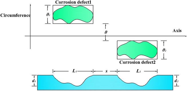
Two corrosion defects of the pipeline are located close to interact each other and the characteristic parameters are shown in Table 1. Fig. 2 shows geometric dimensions of the individual defects. The corrosion defect 1 is located at Pipeline 00:00 position; the corrosion defect 2 and the corrosion defect 1 have the circumferential distance of 30 degrees, and the two defects have no axial spacing.

For the convenience of numerical simulation, the irregular corrosion defects are simplified into rectangular areas, and the size of the rectangular area is determined by the maximum defect depth and the maximum defect length.

For the pipeline, the actual stress-strain curve is used, and the curve is calculated by the constitutive model of Ramberg-Osgood [18].

Table 1Parameters for double corrosion defects

	The relative corrosion depth $(d / t)$	The relative corrosion length $(L / \sqrt{D t})$	The relative corrosion width $(θ / 180^{°})$
Corrosion defect 1	0.4	2.9	0.1
Corrosion defect 2	0.4	2.9	0.1
Notes: $d$ is the measured maximum corrosion pit depth of the corrosion defect, $t$ is the wall thickness of pipeline; $L$ is the allowable maximum longitudinal length; $D$ is the pipe OD; $θ$ is the angle of corrosion defects along the pipeline

Fig. 2Geometric dimensions of the individual defects

Other basic parameters [19] of pipeline steel are shown in Table 2. Data of heat preservation layer and soil refer to data in the references [20, 21].

Table 2Basic parameters of pipeline steel

Density / kg·m^-3	Linear expansion coefficient / mm·(mm·°C)^-1	Thermal conductivity / W·(m·°C)^-1	Specific heat capacity / J·(kg·°C)^-1
7833	1.112×10^-5（20°~50°）	46	750

4.2. Boundary conditions

Because the research object is long-distance transportation pipeline, it can be approximately considered that there is no axial displacement in the pipeline. An axial displacement constraint is imposed on one end of the pipeline and the other end is imposed on its symmetric displacement constraints.

On the basis of the above analysis, a three-dimensional thermal-fluid-solid multi-field coupling mechanical model is established, composed of double corroded pipelines, heat preservation layers and soil, the load boundary conditions and displacement boundary conditions are applied to the model.

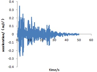
Load boundary conditions: the internal fluid pressure is 4 MPa, the temperature is 48 ℃, and the average velocity is 0.75 m/s. The external atmospheric temperature is 19.4 ℃, the air convection coefficient is 12.5 w/(m²·k), and a constant temperature load of 4 ℃ is applied on the bottom of the constant temperature layer. The pipeline is subjected to the action of EL-centro seismic loading [22], and the action time of seismic loading is 30 s; the direction of the wave action is along the axial direction of pipeline [23], and the curve of acceleration time is shown in Fig. 3.

Displacement boundary conditions: the displacement at the bottom of the simplified rectangular region (constant temperature layer) is completely restrained; the displacement of the connection between the soil’s surface and atmospheric is free; an axial displacement constraint is applied at one end of the cross section of the pipeline, and a symmetric displacement constraint is applied at the other end; the symmetrical displacement constraints are applied to the axial section of pipeline; the displacement constraint is applied on the other side of the rectangular region.

Fig. 3Curve for acceleration time of EL-centro seismic loading

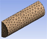
4.3. Mesh model

The structure of pipeline, fluid, heat preservation layer and soil are discretized respectively, and then the whole mesh model is shown in Fig. 4.

5. Analysis of influence factors

In order to study the mechanical properties of corroded pipelines with multi-field coupling effect under seismic loading, the numerical simulation of different fluid temperature, different fluid pressure, different defect characteristics and different types of seismic loading are developed, and the results are analyzed and discussed.

Fig. 4The overall three-dimensional mesh model

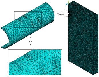
a) Mesh model of solid with double corrosion defects

b) Mesh model of pipeline fluid

5.1. Influence of fluid temperature in pipeline

In the premise of other load boundary conditions and displacement boundary conditions invariant, multi-field couplings numerical simulation for pipelines with double corrosion defects with fluid temperatures of 40 ℃, 48 ℃, 53 ℃ and 60 ℃ are carried out respectively. Curves for the stress, displacement and strain of the corroded pipeline, changed with fluid temperature, are shown in Figs. 5-7 respectively. The maximum strain distribution of the corroded pipeline is shown in Fig. 8.

Fig. 5Curve for stress of corroded pipeline changed with fluid temperature

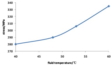
Fig. 6Curve for displacement of corroded pipeline changed with fluid temperature

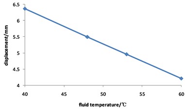
Fig. 7Curve for strain of corroded pipeline changed with fluid temperature

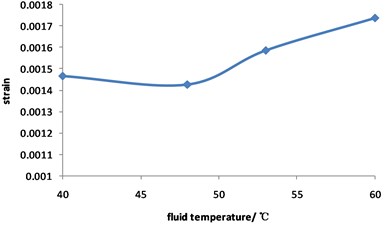
Fig. 5 shows that the pipeline stress increases with the increasing of the fluid temperature. The value of stress is 280 MPa when the fluid temperature is 40 ℃, while the value of stress is 335 MPa when the fluid temperature is 60 ℃, with an increase of 19.6 %.

Fig. 6 shows that with the increase of the fluid temperature, the maximum displacement of the pipeline shows a downward trend. The value of displacement is 6 mm when the fluid temperature is 40 ℃, and drops to 4 mm when the fluid temperature is 60 ℃, with a decrease of 33.3 %.

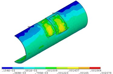
Fig. 7 and Fig. 8 shows that with the increase of fluid temperature, the strain of pipeline presents a steady change and then increases obviously. When the fluid temperature at the top corrosion of pipeline is 40 ℃, the maximum strain with the value of 0.0015; when the fluid temperature exceeds 48 ℃, the maximum strain increases continuously, but the position does not change, and it appears in the corrosion pits near the middle of pipeline. The fluid temperature increases by 50 %, and the strain of the pipeline with double corrosion defects increases by 18.5 %.

Fig. 8Distribution position for maximum strain of corroded pipeline with different fluid temperature

a) Fluid temperature is 40 ℃

b) Fluid temperature is 48 ℃

c) Fluid temperature is 53 ℃

d) Fluid temperature is 60 ℃

5.2. Influence of fluid pressure in pipeline

In the premise of other load boundary conditions and displacement boundary conditions invariant, multi-field couplings numerical simulation for the pipelines with double corrosion defects with fluid pressure of 4 MPa, 5 MPa, 6 MPa and 10 MPa are carried out respectively. Curves for stress, displacement and strain of the corroded pipeline changed with fluid pressure are shown in Figs. 9-11 respectively. The maximum strain distribution of the corroded pipelines is shown in Fig. 12.

Fig. 9 shows that the pipeline stress increases with the increasing of fluid pressure. The value of stress is 290 MPa when the fluid pressure is 4 MPa, while the value of stress is 597 MPa when the fluid pressure is 10 MPa, with an increase of 1.1 times.

Fig. 10 shows that the total displacement of the pipeline is approximately not changed with the increasing of fluid pressure, and the maximum value is about 5 mm all the time.

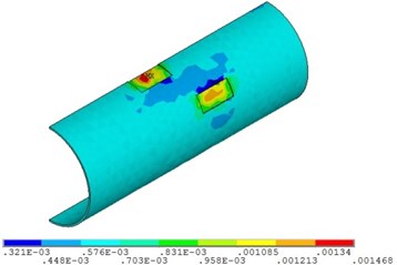
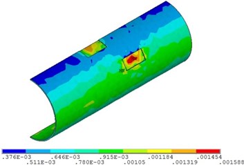
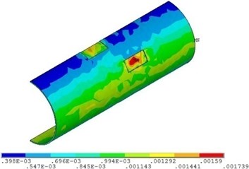
Fig. 11 and Fig. 12 shows that the strain of double corroded pipeline increases with the increasing of fluid pressure, but the position of maximum strain remains unchanged, which is located in the corrosion pit near the middle of pipeline. When the fluid pressure is 4 MPa, the maximum value of double corroded pipeline strain is 0.0014; when the fluid pressure increases to 10 MPa, the maximum value of double corroded pipeline strain is 0.0029.

Fig. 9Curve for stress of corroded pipeline changed with fluid pressure

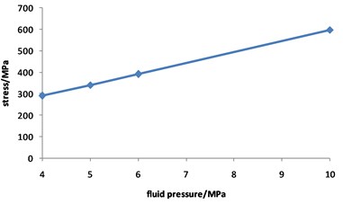
Fig. 10Curve for displacement of corroded pipeline changed with fluid pressure

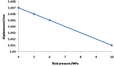
Fig. 11Curve for strain of corroded pipeline changed with fluid pressure

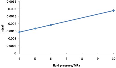
Fig. 12Distribution position for maximum strain of corroded pipeline with different fluid pressure

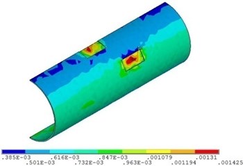
a) Fluid pressure is 4 MPa

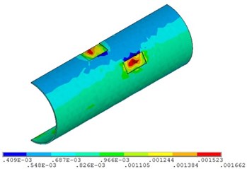
b) Fluid pressure is 5 MPa

c) Fluid pressure is 6 MPa

d) Fluid pressure is 10 MPa

5.3. Influence of corrosion defects characteristics

In the premise of other load boundary conditions and displacement boundary conditions invariant, multi-field couplings numerical simulation for the pipelines with double corrosion defects with different relative corrosion depths, different relative corrosion lengths and different relative corrosion widths under seismic loading are carried out respectively. The calculation conditions are shown in Table 3.

Table 3Calculation conditions of different defect characteristics considering the earthquake time history effect

Case number	Case name	Concrete content
1	Influence of relative corrosion depth	When the other characteristic parameters of the defect are invariant, the multi-field coupling analysis is carried out on the corroded pipeline with the relative corrosion depth of 0.3, 0.4, 0.5 and 0.6 respectively.
2	Influence of relative corrosion length	When the other characteristic parameters of the defect are invariant, the multi-field coupling analysis is carried out on the corroded pipeline with the relative corrosion length of 2.9, 6.2 and 8.2 respectively.
3	Influence of relative corrosion width	When the other characteristic parameters of the defect are invariant, the multi-field coupling analysis is carried out on the corroded pipeline with the relative corrosion width of 0.1, 0.3 and 0.4 respectively.

5.3.1. Influence of relative corrosion depth

According to the multi-field coupling analysis, curves for stress, displacement and strain of pipelines with double corrosion defects changed with the relative corrosion depth under seismic loading are drawn, as shown in Figs. 13-15 respectively. The maximum strain distribution of corroded pipelines is shown in Fig. 16.

Fig. 13Curve for stress of corroded pipeline changed with relative corrosion depth

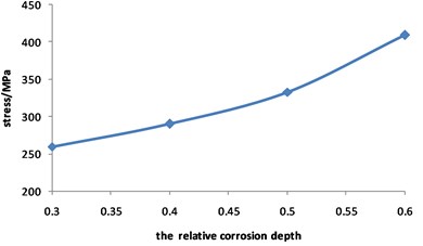
Fig. 14Curve for displacement of corroded pipeline changed with relative corrosion depth

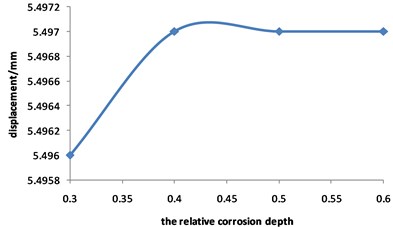
Fig. 15Curve for strain of the pipeline with double corrosion defects changed with the relative corrosion depth

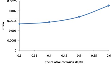
Fig. 13 shows that the pipeline stress increases with the increasing of the relative corrosion depth. The value of stress is 290 MPa when the relative corrosion depth is 0.3, while the value of stress is 409 MPa when the relative corrosion depth is 0.6, with an increase of 57.3 %.

Fig. 14 shows that the total displacement of pipeline is approximately not changed with the increasing of the relative corrosion depth, and the maximum value is always about 5.5 mm.

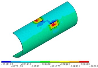
Fig. 15 and Fig. 16 show that the strain of the pipeline with double corrosion defects increases with the increasing of the relative corrosion depth, but the maximum position remains unchanged, which is located in the corrosion pit near the middle of pipeline. When the relative corrosion depth is 0.3, the maximum value of the pipeline with double corrosion defects is 0.0013; when the relative corrosion depth is 0.6, the maximum value of the corroded pipeline strain is 0.0023.

Fig. 16Distribution position for maximum strain of the pipeline with double corrosion defects with different relative corrosion depth

a) Relative corrosion depth is 0.3

b) Relative corrosion depth is 0.4

c) Relative corrosion depth is 0.5

d) Relative corrosion depth is 0.6

5.3.2. Influence of relative corrosion length

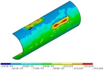
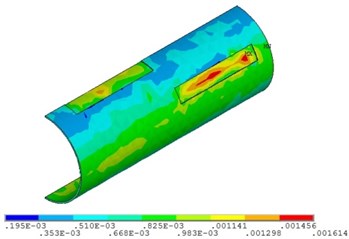
According to the multi-field coupling analysis, curves for stress, displacement and strain of the pipeline with double corrosion defects changed with the relative corrosion length under seismic loading are drawn, as shown in Figs. 17-19 respectively. The maximum strain distribution of the corroded pipeline is shown in Fig. 20.

Fig. 17Curve for stress of corroded pipeline changed with relative corrosion length

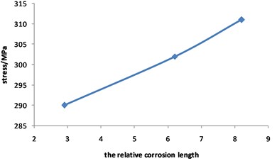
Fig. 18Curve for displacement of corroded pipeline changed with relative corrosion length

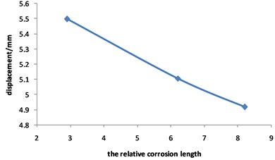
Fig. 17 shows that the pipeline stress increases with the increasing of the relative corrosion length. The value of stress is 290 MPa when the relative corrosion length is 2.9, while the value of stress is 311 MPa when the relative corrosion length is 8.2, with an increase of 7.2 %.

Fig. 18 shows that the maximum displacement of the pipeline with double corrosion defects decreases slightly with the increase of the relative corrosion length, and it can be approximately considered that the displacement does not change with the increase of the relative corrosion length.

Fig. 19Curve for strain of the pipeline with double corrosion defects changed with the relative corrosion length

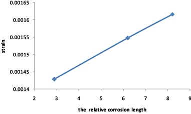
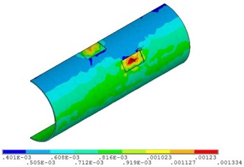
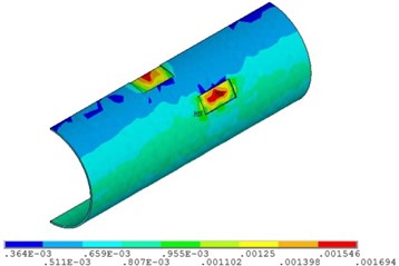
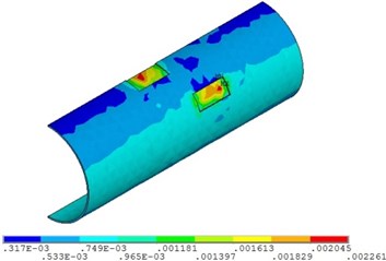
Fig. 20Distribution position for maximum strain of the corroded pipeline with different relative corrosion lengths

a) Relative corrosion length is 2.9

b) Relative corrosion length is 6.2

c) Relative corrosion length is 8.2

Fig. 19 and Fig. 20 show that the strain of the pipeline with double corrosion defects increases with the increasing of the relative corrosion length, but the maximum position remains invariant, which is located in the corrosion pit near the middle of pipeline. When the relative corrosion length is 2.9, the maximum value of the strain of the pipeline with double corrosion defects is 0.0014; when the relative corrosion length is 8.2, the maximum value of the corroded pipeline strain is 0.0016.

5.3.3. Influence of relative corrosion width

According to the multi-field coupling analysis, curves for stress, displacement and strain of the pipeline with double corrosion defects changed with the relative corrosion width under seismic loading are drawn, as shown in Figs. 21-23 respectively. The maximum strain distribution of the corroded pipeline is shown in Fig. 24.

Fig. 21Curve for stress of corroded pipeline changed with relative corrosion width

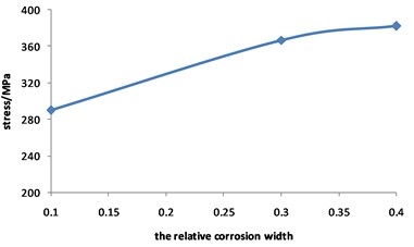
Fig. 22Curve for displacement of corroded pipeline Changed with relative corrosion width

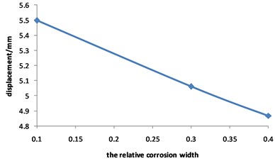
Fig. 23Curve for strain of the corroded pipeline changed with the relative corrosion width

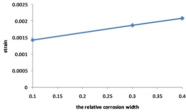
Fig. 24Distribution position for maximum strain of the pipeline with double corrosion defects with different relative corrosion widths

a) Relative corrosion width is 0.1

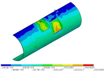
b) Relative corrosion width is 0.3

c) Relative corrosion width is 0.4

Fig. 21 shows that the pipeline stress increases with the increasing of the relative corrosion width. The value of stress is 290 MPa when the relative corrosion width is 0.1, while value of stress is 382 MPa when the relative corrosion width is 0.4, with an increase of 31.7 %.

It can be seen from Fig. 22 that the maximum displacement of the pipeline with double corrosion defects decreases slightly with the increase of the relative corrosion width, and it can be approximately considered that the displacement does not change with the increase of the relative corrosion width.

Fig. 23 and Fig. 24 show that the strain of the pipeline with double corrosion defects increases with the increasing of the relative corrosion length, and the maximum position changes. When the relative corrosion width is 0.1, the maximum value is 0.0014, located in the corrosion pit near the middle of pipeline; when the relative width is up to 0.4, the maximum value is 0.0021, located on the top of pipeline. Thus, the wider the relative corrosion width is, the defects at the top of pipeline are more likely to fail.

Fig. 25Curve for acceleration time-history of Taft seismic loading

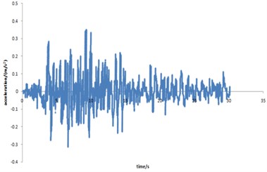
Fig. 26Curve for acceleration time-history of spux seismic loading

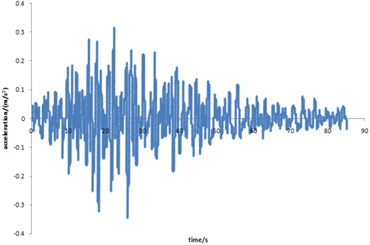
Fig. 27Distribution position for maximum strain of acceleration time-history with different types of seismic loading

a) EL-centro seismic loading

b) Taft seismic loading

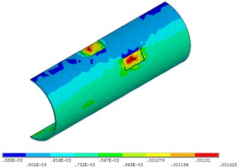
c) Spux seismic loading

5.4. Influence of seismic loading

In the premise of other load boundary conditions and displacement boundary conditions are invariant, EL-centor seismic loading, Taft seismic loading and spux seismic loading are applied to the pipelines with double corrosion defects respectively. In order to make the calculation results comparable, the first thirty second acceleration of each seismic loading are applied to the mechanical model. The acceleration time history curves of Taft seismic loading and spux seismic loading are shown in Figs. 25-26 respectively. The maximum strain distribution of the corroded pipeline is shown in Fig. 27.

Fig. 27 shows that when the time of the seismic loading action is 30 seconds, the pipeline strain does not change with the change of different seismic loading. This is due to the short time and the great intensity of earthquake.

6. Conclusions

For corroded pipelines in cold regions, considering the nonlinear properties of the material of pipeline steel and the frost heave characteristic of soil, the three-dimensional thermal-fluid-solid coupling mechanics model is established, method by FEM (finite element method). The model is applied to do the dynamic response analysis for corroded pipelines under seismic loading, and the different influence factors on the mechanical properties of pipelines are then discussed.

The results show that for the different influence factors, the relative corrosion depth, the fluid pressure and the fluid temperature have obvious influence on the mechanical characteristics of the pipeline with double corrosion defects, the relative corrosion width comes second, and the relative corrosion length has less influence on it. The mechanical characteristics of pipeline do not change with different seismic loading. When the relative corrosion depth increases by 1 times, the strain increases by 69.4 %; when the fluid pressure increases by 1.5 times, the strain increases by about 1 times; when the fluid temperature increases by 50 %, the strain increases by 18.5 %.

The three-dimensional multi-field coupling mechanics model and the calculation method established in this paper provide an analytical method and theoretical basis for the evaluation of pipeline integrity in cold regions. In order to ensure that the buried pipelines in cold regions operate safely and steadily, the fluid pressure, fluid temperature and the relative corrosion depth should be the key factors monitored in the process of pipeline integrity management, and targeted measures of maintenance should be taken.

References

Fang J. P., Duan Q. Q. Failure analysis of oil and gas pipeline in low temperature permafrost area. Oil and Gas Transportation and Storage, Vol. 34, Issue 3, 2016, p. 7-10.

Search CrossRef
Clark J., Phillips R. Centrifuge modeling of frost heave of arctic gas pipelines. The 8th International Conference on Permafrost, 2003.

Search CrossRef
Palmer A. C., Williams P. J. Frost heave and pipeline upheaval buckling. Canadian Geotechnical Journal, Vol. 40, Issue 1, 2003, p. 1033-1038.

Publisher
Zhang K., Lian Z. H., Xia Y. B., et al. Analysis of thermal deformation of buried pipeline in permafrost zone. Petroleum Engineering Construction, Vol. 32, Issue 4, 2006, p. 4-6.

Search CrossRef
Li S. L. Influence Analysis for Frozen Soil Expansion on Stress Change of Regulating Station Pipeline. Capital University of Economics and Business, Beijing, 2014.

Search CrossRef
Tang M. C. Calculation of Thermal-Stress on Shallow-buried Oil pipeline in Cold Area. Tongji University, Shanghai, 2007.

Search CrossRef
Li K., Wang Z. F., Xiang W. D., et al. Mechanical analysis of frost heaving of pipeline in gas offtake station. Oil and Gas Storage and Transportation, Vol. 30, Issue 8, 2011, p. 652-656.

Search CrossRef
Fokeeva M., Radina E. Influence of permafrost conditions on gas mains stability in cryolithozone. Journal of Glaciology and Geocryology, Vol. 26, 2004, p. 215-219.

Search CrossRef
Li Y. H., Wu W., Hao J. Q., et al. Determination of the wall thickness for designing the steel pipe in frozen ground along the China-Russia crude oil pipeline route. Journal of Glaciology and Geocryology, Vol. 30, Issue 4, 2008, p. 605-610.

Search CrossRef
Zhu Q. J., Chen Y. H., Liu T. Q., et al. Finite element analysis of fluid-structure interaction in buried liquid-conveying pipeline. Journal of Central South University of Technology, Vol. 15, Suppl. 1, 2008, p. 307-310.

Publisher
Shao G. B. Numerical analysis for oil pipeline subjected to earthquake liquefaction-induced lateral spreading. Advanced Materials Research, Vols. 243-249, 2011, p. 3804-3807.

Publisher
Hu Y. W. Study on the Effect of Site Subsidence on Buried Pipeline. Institute of Engineering Mechanics, China Earthquake Administration, Harbin, 2008.

Search CrossRef
Fang J. P. Accident Analysis of domestic and international oil and gas pipelines. Oil and Chemical Equipment, Vol. 19, 2016, p. 90-93.

Search CrossRef
Yu H. Forward and Reverse Transporting Optimization Technology Research of Su Cuo Oil Pipeline. Northeast Petroleum University, Daqing, 2016.

Search CrossRef
Yang S. M., Tao W. Q. Heat Transfer. Higher Education Press, Beijing, 2006, p. 42-44.

Search CrossRef
Shuai J. Pipeline Mechanics. Science Press, Beijing, 2010, p. 198-199.

Search CrossRef
Sun H. Study and Application on Coupled Fluid-Solid and Heat-Fluid-Solid Theories of Sand Control Technology in Weakly Consolidated Reservoirs. China University of Petroleum, Qingdao, 2008, p. 87-89.

Search CrossRef
Zhao X., Ma Y. X., Wu Z. F., et al. Study on security of long-distance transport X52 pipeline in suspended state. Mechanical Science and Technology for Aerospace Engineering, Vol. 34, Issue 10, 2015, p. 1589-1593.

Search CrossRef
China National Standardization Management Committee. GB150-2011, Pressure Vessel, 2012.

Search CrossRef
Li N. S., Xie L. H., Chen X. H. Frozen heaving of frost soli bed of shallow buried oil pipeline in cold region. Structural Engineers, Vol. 24, Issue 1, 2008, p. 35-40.

Search CrossRef
Li H. The Study on the Stability of the Embankment Upon the Slope under Earthquake Load in Permafrost Area. Beijing Jiaotong University, Beijing, 2010.

Search CrossRef
Wang H. L., Chen Q. J. Comparison of wave- passage effect on large-span connective structures under different seismic waves. Journal of Jiamusi University (Natural Science Edition), Vol. 31, Issue 4, 2013, p. 510-515.

Search CrossRef
Cao W. R., Qi L., Cao X. F. Numerical analysis of dynamic response of submarine pipeline under seismic loading. Proceedings of China Oil and Gas Forum – A Special Symposium on Oil and Gas Pipeline Technology, 2014, p. 659-663.

Search CrossRef

About this article

Received

21 October 2017

Accepted

05 January 2018

Published

15 August 2018

SUBJECTS

Seismic engineering and applications

DOI

https://doi.org/10.21595/jve.2018.19300

Keywords

corroded pipelines

cold regions

seismic loading

multi-field coupling

influence factors

Acknowledgements

This work was partly supported by National Natural Science Foundation of China (No. 51674086).

This is an open access article distributed under the Creative Commons Attribution License, which permits unrestricted use, distribution, and reproduction in any medium, provided the original work is properly cited.

Previous article in issue Previous Next article in issue Next

Research article

2023 08 03

Determining tunnel stability across fault zones under seismic loading based on load/unload response ratio theory

Qiang Hui, Feng Gao, Xukai Tan, Dongmei You

Research article

2023 02 17

Shaking table tests of large cross-sectional multi-crack tunnel linings

Dongmei You, Feng Gao

Research article

2021 06 28

Research on key technology of automatic loading and unloading of dual pipe directional drilling

Kun Li, Yafeng Yao

Research article

2017 11 15

Dynamic response and limit analysis of buried gas pipeline under ground consolidation load

Taolong Xu, Jian Mao, Yanhua Liu, Anlin Yao

Q. Z. Li, Y. Liu, L. X. Wei, and M. Luo, “Multi-field coupling dynamic response analysis of pipelines with double corrosion defects under seismic loading in cold regions,” Journal of Vibroengineering, Vol. 20, No. 5, pp. 2111–2127, Aug. 2018, https://doi.org/10.21595/jve.2018.19300

Copy Extrica

Copied to clipboard!

TY  - JOUR
DO  - 10.21595/jve.2018.19300
UR  - https://doi.org/10.21595/jve.2018.19300
TI  - Multi-field coupling dynamic response analysis of pipelines with double corrosion defects under seismic loading in cold regions
T2  - Journal of Vibroengineering
AU  - Li, Qiao Zhen
AU  - Liu, Yang
AU  - Wei, Li Xin
AU  - Luo, Min
PY  - 2018
DA  - 2018/08/15
PB  - JVE International Ltd.
SP  - 2111-2127
IS  - 5
VL  - 20
SN  - 1392-8716
SN  - 2538-8460
ER  - 

Copy Ris

Copied to clipboard!

@article{Li_2018,
	doi = {10.21595/jve.2018.19300},
	url = {https://doi.org/10.21595/jve.2018.19300},
	year = 2018,
	month = {aug},
	publisher = {{JVE} International Ltd.},
	volume = {20},
	number = {5},
	pages = {2111--2127},
	author = {Qiao Zhen Li and Yang Liu and Li Xin Wei and Min Luo},
	title = {Multi-field coupling dynamic response analysis of pipelines with double corrosion defects under seismic loading in cold regions},
	journal = {Journal of Vibroengineering}
}

Copy Bibtex

Copied to clipboard!

[1]Q. Z. Li, Y. Liu, L. X. Wei, and M. Luo, “Multi-field coupling dynamic response analysis of pipelines with double corrosion defects under seismic loading in cold regions,” Journal of Vibroengineering, vol. 20, no. 5, pp. 2111–2127, Aug. 2018, doi: 10.21595/jve.2018.19300.

Copy IEEE

Copied to clipboard!

Li, Qiao Zhen, Yang Liu, Li Xin Wei, and Min Luo. “Multi-Field Coupling Dynamic Response Analysis of Pipelines with Double Corrosion Defects under Seismic Loading in Cold Regions.” Journal of Vibroengineering 20, no. 5 (August 15, 2018): 2111–27. https://doi.org/10.21595/jve.2018.19300.

Copy Chicago

Copied to clipboard!

Multi-field coupling dynamic response analysis of pipelines with double corrosion defects under seismic loading in cold regions

Abstract

1. Introduction

2. Physical model

3. Multi-field coupling mathematical model

3.1. Temperature field control equation

3.2. Multi-field coupling equation

4. Finite element model

4.1. Basic data

4.2. Boundary conditions

4.3. Mesh model

5. Analysis of influence factors

5.1. Influence of fluid temperature in pipeline

5.2. Influence of fluid pressure in pipeline

5.3. Influence of corrosion defects characteristics

5.3.1. Influence of relative corrosion depth

5.3.2. Influence of relative corrosion length

5.3.3. Influence of relative corrosion width

5.4. Influence of seismic loading

6. Conclusions

References

About this article

Related Articles