Abstract
When fault arises in the rolling element bearing, the time-domain waveform of fault vibration signal will take on the characteristic of cyclostationarity, and the spectral correlation (SC) or spectral correlation density (SCD) basing on second order cyclic statistic is an effective cyclostationarity signal processing method. However, when the fault signal is surrounded by strong background noise, the traditional signal processing methods such envelope demodulation analysis and SC would not work effectively. The paper improves the SC method and a new time-frequency analysis method naming improved spectral correlation (ISC) is proposed. The proposed method is much more noise-resistant than SC through the verification of simulation analysis results. Besides, it takes on modulation phenomenon usually when fault arises in the rolling element bearing and the aim of fault feature extraction is to extract the fault characteristic frequency only or cyclic modulation frequency and the modulated frequency or carrier frequency buried in the object vibration signal is neglected. So, the paper improves the ISC further and the improved ISC (IISC) is proposed. The IISC will extract the modulation frequency only and it has the advantages of much clearer expression effect and better extraction effect. The effectiveness and feasibility of the proposed method are verified through the three kinds of fault (inner race fault, outer race fault and rolling element fault) of rolling element bearing. Besides, the advantages of the proposed method over the other relative time-frequency analysis methods such as ensemble empirical mode decomposition (EEMD) and spectral kurtosis (SK) are also presented in the paper.
1. Introduction
As the common used part and one of the most critical component in the rotating machinery, the study on the effective fault feature extraction method of rolling element bearing prior to its complete failure occurring in the practical engineering application is very important and necessary. However, it is unable to extract the fault feature of rolling element bearing using traditional signal processing methods if the impulsive characteristic of the fault signal is buried by strong background noise. Besides, the existed signal attenuation phenomenon between the fault source and the sensor collecting the fault signal will cause the failure result of fault feature extraction. Time-frequency analysis is an effective signal processing method and has been used widely in fault feature extraction of rotating machinery. In paper [1], the time-frequency methods such as wavelet packet decomposition and short time Fourier transform are used in selecting the most impulsive frequency bands and the effective fault feature vector is extracted. Then the extracted vectors are used as the training and test input of the intelligent algorithm-Linear Discriminant Analysis, and satisfactory fault classification results of rolling element bearing are obtained at last. A new fractional lower order stockwell transform time frequency representation method employing fractional lower order moment and inverse FLOST were proposed in paper [2] and used in processing mechanical bearing fault signal, and the excellent performance of the proposed method is presented through experiment verifications. The empirical wavelet transform (EWT) was improved and an adaptive parameterless EWT (AEWT) method was proposed in paper [3]. The proposed method was applied to fault diagnosis of rotor system with local rubbing and satisfactory analysis results were obtained at last. The time-frequency representation method, Particle Swarm Optimization and artificial neural network were combined and a new classification method for the fault diagnosis of induction machine was proposed in paper [4]. By combining the concepts of time-frequency manifold and image template matching, a novel time-frequency manifold correlation matching method was proposed in paper [5] to enhance the ability of identification the periodic faults signal, and the proposed method is verified to be superior to the traditional enveloping method through the analysis results of gearbox fault signal. The Hilbert versus Concordia transform [6] was used in monitoring the stator current of the three-phase machine in the time-frequency domain. Three kinds of time-frequency analysis method naming short time Fourier transform, continuous wavelet transform and Hilbert Huang transform were used to analyze the rotor startup vibrations in paper [7], and the performances comparison of them were presented in the paper. The energy concentration level is an important indicator for valuing the quality of time-frequency analysis result. A generalized stepwise demodulation transform was proposed in paper [8] to improve the energy concentration level problem existing in common used time-frequency analysis methods. Noise suppression and resolution improvement are the remaining problems for the time-frequency analysis method application in rolling bearing fault feature extraction. To solve the problem, Xu J and other authors proposed a novel time-frequency correlation matching and reconstruction method to enhance the fault feature extraction ability of the time-frequency analysis method [9]. The non-Gaussian and nonlinear gear vibration signal collected in the running time is analyzed difficultly in frequency or time domain, and Liu W. R. and other authors proposed a hybrid time-frequency analysis method by combining the Mexican hat wavelet filter de-noising method with the auto term window method [10]. The proposed method could not only de-noise the noise jamming in the raw vibration signal but also extract the gear fault features perfectly. In this paper, a noise-resistant time-frequency method is proposed and used in fault diagnosis of rolling element bearing. The feasibility and effectiveness of the proposed method are verified through simulation and experiment.
The paper is organized as follows. Section 2 is dedicated to the basis theory of SC, ISC and IISC. Section 3 is the simulation verifying the effectiveness and feasibility of the proposed method. In Section 4 the experimental analyzed results of rolling element bearing’ three kinds of fault (inner race faults, outer race fault and rolling element faults) are presented. Besides, in Section 5 the analyzed experimental results using EEMD and SK methods are also presented and the advantages of the proposed method over them are verified further. The conclusions obtained from the above results are given in Section 6.
2. The theory of SC and the improved methods
2.1. SC
The basis theory of SC is cyclostationarity which has been existing for several decades [11, 12]. A random signal can be defined as stationary at th order if its time-domain th-order moment will not vary according to the time , and a random signal can be defined as having the characteristic of cyclostationarity at th-order if the period of its time domain th-order moment is a periodical function of time . The fundamental frequency of the periodicity is called cyclic frequency of the signal [13].
The first-order cyclostationarity: The first order moment, i.e. the mean, is time periodical if the following equation is satisfied:
The second-order cyclostationarity: The signal is defined as second-order cyclostationarity if its autocorrelation function satisfies the following equation for any :
where is the cyclic period and is the corresponding fundamental cyclic frequency.
The Fourier series of equation can be represented as following:
where are the Fourier coefficient.
Spectral coherence theory: The spectral correlation density function of a cyclostationarity signal is defined as the Fourier transform of the signal’ cyclic autocorrelation function :
where is the cyclic frequency and is the spectral frequency.
In corresponding, the spectral coherence function of is defined as:
with being the time-averaging operator:
is the time average correlation coefficient of between the two frequencies at and . Further, the absolute value of satisfies:
With the value being much closer to 1 means the stronger linear dependence between the two spectral lines locating at frequencies and , and vice versa. If an observed signal exhibits cyclostationarity, there must be existing non-zero , and the corresponding space between the two correlated components must be one of the cyclic frequencies .
The interrelation of the second-order cyclostationarity processes can be referred to Fig. 1.
2.2. ISC
Considering a sine signal with frequency is modulated by the sine signal with frequency and its harmonic is shown in Eq. (8):
In Eq. (8), is the random white noise. The frequency spectrum of the signal shown in Eq. (8) is presented in Fig. 2. The center frequency is the frequency of carrier signal, and the frequency with its harmonics of the modulating signal locates symmetrically from by cyclic frequency .
Fig. 1The cyclostationarity processes
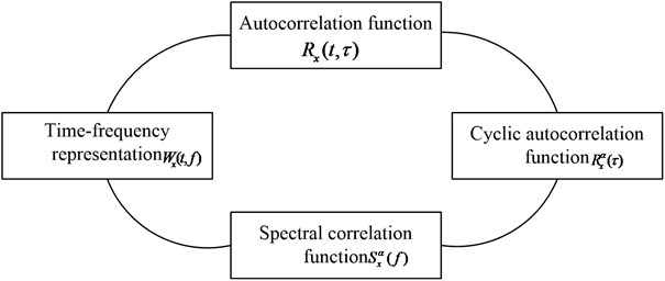
Fig. 2The structure diagram of the side band filter
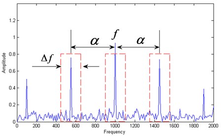
Commonly a side band filter whose structure diagram is shown in Fig. 2 is used to filter the carrier and modulating signal. Ideally, the object signal with only small amount of noise will be obtained by the above side band filter and the filtered signal can be represented by following equation:
where represents the filtered signal in the narrow band frequency scale . The relationship of the three spectrum components can be calculated by the output of the filter, and the calculated result is used an indicator to reflect the modulation phenomenon. The SC is the common used indicator:
where represents the complex envelope of the filtered signal by using the filter shown in Fig. 2 in the narrow band frequency scale . The can be represented by the following equation:
The relationship between and can be calculated using the following equation:
Same as the Eq. (2), the SC can also be calculated by the following equation as the substitution of Eq. (10):
So, the SC can also be represented as following:
Based on the above equations and Fig. 1, the SC between and can be calculated as following:
Analogically, the SC between and can be calculated as following:
In order to obtain the relationships of the three spectrum components spaced by the cyclic frequency , the above two equations are multiplied and the ISC is obtained:
where represents the inner product of SC. The ISC spectral reflects the relationship between the carrier frequency and the modulating frequency .
2.3. IISC
As shown in Eq. (17), the ISC is the function with respect to carrier frequency and modulating frequency . However, the modulating frequency is the extraction objection and the carrier frequency is neglected usually, so the ISC is improved further here and the IISC is proposed which can be calculated using the following equation:
The advantage of IISC over ISC is that the analysis result of the former is much more intuitionistic than the latter. Besides, the computational efficiency of the former is also higher than the latter due to the reason that the latter will not only extracts the carrier frequency but also extracts the modulating frequency, and the former only extracts the modulating frequency. These two advantages will be verified in the simulation and experiment.
3. Simulation
Use the signal shown in Eq. (19) to simulate the modulation phenomenon when fault arises in the rolling element bearing:
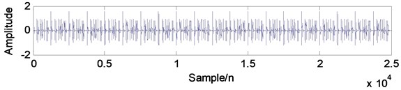
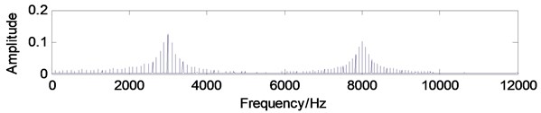
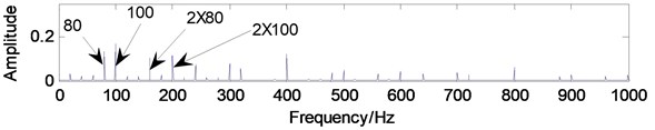
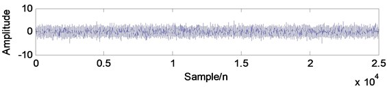
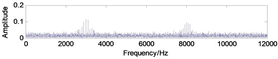
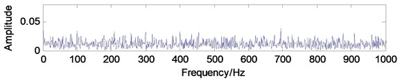
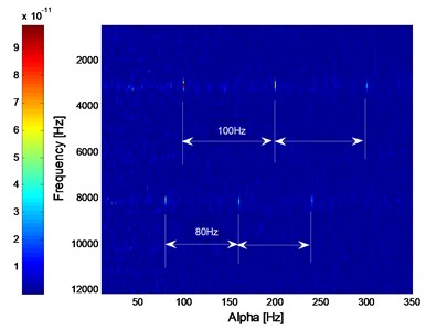
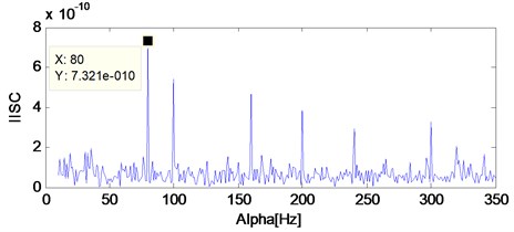
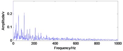
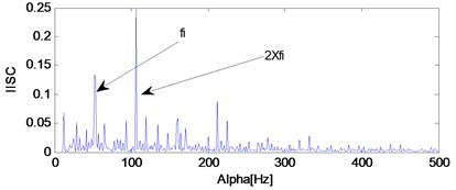
where 1/25000, 1:25000, , , and the two carrier frequencies are 3 kHz and 8 kHz respectively, and the corresponding modulating frequencies are 100 Hz and 80 Hz. The time-domain waveform, frequency spectrum and the envelope demodulation spectrum of the simulation signal are shown in Fig. 3(a), (b) and (c) respectively. The corresponding SC and ISC spectral analysis results of the simulation signal are shown in Fig. 4(a) and (b), and it is evident that the SC and ISC both could extract the fault feature frequency successfully when there is not noise interference. Fig. 5 is the IISC spectral analysis result which is more intuitionistic than the SC and ISC spectral shown in Fig. 4: The object modulating frequencies 80 Hz and 100 Hz are only shown in the Fig. 5 which is very intuitionistic. Besides, the computation consuming time of IISC is only half of the computation consuming time of ISC: The latter calculates the carrier frequency and modulating frequency simultaneously while the former calculates the modulating frequency only.
Fig. 3The simulation signal: a) time-domain waveform, b) frequency-domain waveform, c) envelope demodulation spectrum
a)
b)
c)
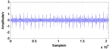
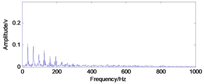
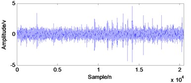
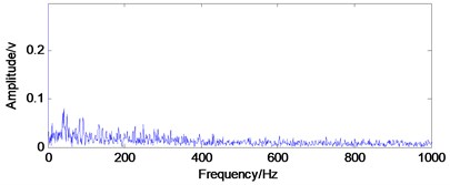
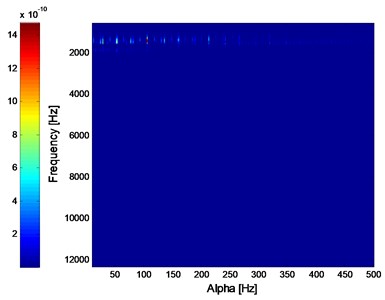
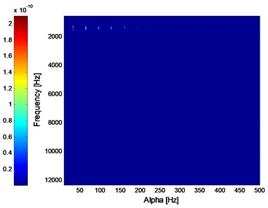
Add white noise into the signal shown in Fig. 3(a) and the noised signal is shown in Fig. 6(a). The frequency-domain waveform and envelope demodulation spectrum of the noised signal are given in Fig. 6(b) and (c) from which the fault characteristic frequencies could not be extracted due to the influence of white noise. The SC and ISC analysis results of the noised signal are shown in Fig. 7 from which the fault characteristic frequency could not be extracted by SC, but the fault characteristic frequency can be extracted successfully by ISC. The above analysis results verify that the ISC is a noise-resistant time-frequency method. Besides, the IISC of the noised signal is shown Fig. 8 and the extracted result is more intuitional than the results being shown in Fig. 7 which verifies that the IISC not only owns the virtue of noise-resistant but also has the advantage of more intuitional than ISC. Besides, the computation efficiency of IISC is also higher than ISC through statistics.
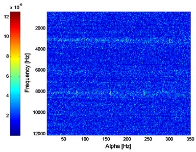
Fig. 4The SC and ISC analysis result of the simulation signal: a) SC, b) ISC
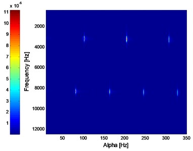
a) SC
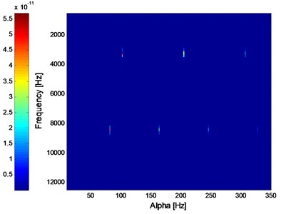
b) ISC
Fig. 5The IISC analysis result of the simulation signal
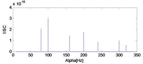
Fig. 6The simulation signal added with white noise: a) time-domain waveform, b) frequency-domain waveform, c) envelope demodulation spectrum
a)
b)
c)
Fig. 7The SC and ISC analysis result of the simulation signal added with white noise: a) SC, b) ISC
a) SC
b) ISC
Fig. 8The IISC analysis result of the simulation signal added with white noise
4. Experiment
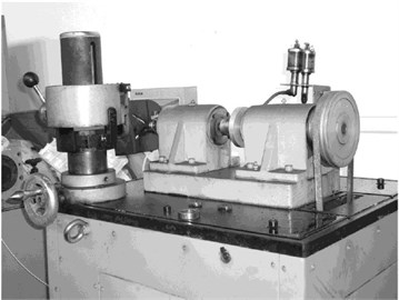
The bearing fault vibration signals are collected on the test rig shown in Fig. 9. The three kinds of different fault (inner race fault, outer race fault and ball fault) are carried out on the test rig. As shown in Fig. 9, the two ends of the rotor are supported by support devices and test rolling element bearings. The test rig is equipped with hydraulic positioning and clamping device which are used to fix the outer race of the test rolling element bearing in the test process. The experimental platform is driven by an AC motor, and the rotor is driven by the coupling. In the test processing, the outer race of the test bearings are fixed on the support devices, and the inner race rotates with the working shaft synchronously. The rotating speed of the shaft is 720 r/rpm. The type of the test bearing is GB203. The parameters and the relative fault characteristic frequencies of the test rolling element bearings are shown in table1. The sampling frequency is 25.6 kHz.
Fig. 9The test rig
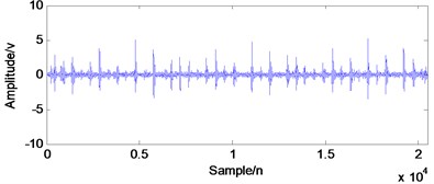
The inner race, rolling element and outer race of the test rolling bearings are eroded with very tiny point corrosions respectively using Electrical Discharge Machining (EDM) technology to simulate the three kinds of fault of the rolling bearing. The time-domain waveforms of the corresponding three states and their corresponding envelope demodulation spectrums are shown in Fig. 10.
Table 1The parameters and theory fault characteristic frequencies of the test bearing
Type | Pitch diameter (mm) | Ball diameter (mm) | Ball number | Contact angle |
GB203 | 28.5 | 6.747 | 7 | 0 |
Characteristic frequency (CF) | Calculation equation | Results (Hz) | ||
Rotating CF | 12 | |||
Ball CF | 47.8 | |||
Inner race CF | 51.9 | |||
Outer race CF | 32.1 | |||
Cage CF | 4.6 | |||
Fig. 10The time-domain waveforms with their envelope spectrums of the experiment: a) time-domain waveform of inner race fault, b) envelope spectrum of a), c) time-domain waveform of outer race fault, d) envelope spectrum of c), e) time-domain waveform of element fault, f) envelope spectrum of e)
a) Time-domain waveform of inner race fault
b) Envelope spectrum of a)
c) Time-domain waveform of outer race fault
d) Envelope spectrum of c)
e) Time-domain waveform of element fault
f) Envelope spectrum of e)
As shown in Fig. 10(b) and (d), when fault arises in the rolling element bearing, the inner race and outer race fault characteristic frequencies could be extracted successfully by using the envelope demodulation analysis method. However, the envelope demodulation method would not work effectively as shown in Fig. 10(f) when fault arises on the rolling ball due to the influence of the cage frequency and its harmonics. Besides, the background noise will also decrease the effectiveness of envelope demodulation spectrum in fault feature extraction.
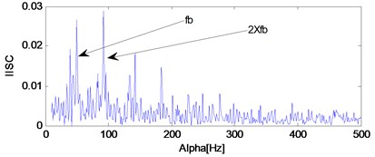
The corresponding ISC spectral of the three states’ vibration signals are shown in Fig. 11. As shown in Fig. 11(a) and (b), the ISC will extract the fault feature of bearing’ inner race fault and outer race fault. However, it would not also work effective same as envelope demodulation method as shown in Fig. 10(f) when fault arises on the balling.
Apply IISC to the fault signal of the three states and the analysis results are shown in Fig. 12. Same as ISC, the IISC will not only work effective when fault arises in inner race or outer race, but also will work effective when fault arises in the rolling ball as shown in Fig. 12(c) which verifies the advantage of IISC over the methods of ISC and SC. The reason can be attributed to the theory of IISC as stated in the above section: it only pays concern to the modulating frequency and neglects the carrier frequency.
5. Comparison
The ensemble empirical mode decomposition (EEMD) [14, 15] is a relative new time-frequency analysis method originating from empirical mode decomposition (EMD). In order to verify the advantages of ISC and IISC, the EEMD analysis result of the signal shown in Fig. 10(e) are presented as following.
Fig. 11The ISC analysis results of the experimental signals: a) the ISC of the signal shown in Fig. 10(a), b) the ISC of the signal shown in Fig. 10(c), c) the ISC of the signal shown in Fig. 10(e)
a) The ISC of the signal shown in Fig. 10(a)
b) The ISC of the signal shown in Fig. 10(c)

c) The ISC of the signal shown in Fig. 10(e)
Firstly, Apply EEMD to the signal shown in Fig. 10(e) and several intrinsic mode functions (imfs) are obtained as shown in Fig. 13. Then calculate kurtosis values of the obtained imfs and select imf owing the biggest kurtosis value as the object for further analysis because it contains the most amount of transient impulse components. At last, apply envelope demodulation spectrum to the selected imf and the result is shown in Fig. 14. The fault feature could not be extract by EEMD method: the ball fault characteristic frequency (47.8 Hz) with its harmonics are not extracted successfully as shown in Fig. 14 because the spectral lines in Fig. 14 are chaotic and the ball fault characteristic frequency could not be identified. However, the ball fault characteristic frequency (47.8 Hz) with its harmonics could be extracted perfectly by using the proposed method as shown in Fig. 12(c).
Fig. 12The ISC analysis results of the experimental signals: a) the ISC of the signal shown in Fig. 10(a), b) the ISC of the signal shown in Fig. 10(c), c) the ISC of the signal shown in Fig. 10(e)
a) The IISC of the signal shown in Fig. 10(a)
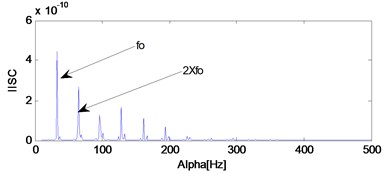
b) The IISC of the signal shown in Fig. 10(c)
c) The IISC of the signal shown in Fig. 10(e)
SK is a powerful time-frequency analysis tool to detect the transient components in vibration signals and has been widely studied and applied in the rotating machine diagnostics [16].
Fig. 13The EEMD analysis results of the signal shown in Fig. 10(e)
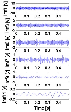
a)
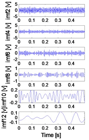
b)
Fig. 14The envelope demodulation spectral analysis imf4 shown in Fig. 13
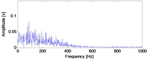
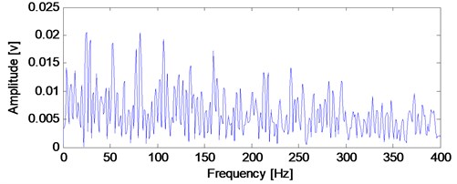
The kurtogram of SK of the original signal shown in Fig. 10(e) is shown in Fig. 15 and the envelope result of the filtered signal basing on the SK analysis shown in Fig. 15 is shown in Fig. 16. It can be seen that the extraction result using SK method is not obvious enough compared with the proposed method: The ball fault characteristic frequency (47.8 Hz) with its harmonics could be identified clearly based on Fig. 16 using SK as compared with the extracted result as shown in Fig. 12(c).
Fig. 15The SK spectral of the signal shown in Fig. 10(e)
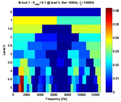
Fig. 16The envelope demodulation spectrum of the filtered ball fault signal basing on SK analysis shown in Fig. 15
6. Conclusions
Basing on the property of cyclostationarity when fault arises in the rolling element bearing, the paper improves the spectrum correlation (SC) or spectrum correlation density (SCD) basing on second order cyclic statistic and proposes a new time-frequency analysis method naming improving spectrum correlation (ISC). When the impulsive characteristic of the signal is evident, the SC and ISC methods both can extract the fault feature easily and this conclusion is deduced by the simulation analysis. Besides, when fault arises in the inner race or outer race of the rolling element bearing, the impulsive characteristic of the two kinds of fault is relative evidently, and the ISC method could also extract the fault feature successfully. However, when fault arises on the rolling element, the signal impulsive feature is surrounded by other interference such as rotating frequency signal with its harmonics, the cage frequency signal with its harmonics and so on, and the ISC methods would not work. It usually takes on modulation phenomenon when fault arises in rolling bearing, and the aim of fault diagnosis is to extract the fault characteristic frequency or cyclic modulation frequency only and neglect the modulated frequency or carrier frequency, so the ISC method is improved further and the integrated improving spectrum correlation (IISC) is proposed. The IISC method not only owns the virtues of ISC, but also could extract the modulation frequency only which has the advantages of clearer expression effect and much better extraction effect. The above stated is verified through simulation and rolling bearing’s three fault types (inner race fault, outer race fault and ball fault).
The analysis results using EEMD and SK methods are also presented in the paper to verify the advantages of the proposed methods further.
References
-
Attoui I., Fergani N., Boutasseta N., Oudjani B. A new time-frequency method for identification and classification of ball bearing faults. Journal of Sound and Vibration, Vol. 397, 2017, p. 241-265.
-
Long J. B., Wang H. B., Zha D. F. Applications of fractional lower order S transform time frequency filtering algorithm to machine fault diagnosis. Plose One, Vol. 12, 2017, p. 4.
-
Zhang J. D., Pan H. Y., Yang S. B. Adaptive parameterless empirical wavelet transform based time-frequency analysis method and its application to rotor rubbing fault diagnosis. Signal Processing, Vol. 130, 2017, p. 305-314.
-
Medoued A., Lebaroud A., Laifa A., Sayad D. Classification of induction machine faults using time frequency representation and particle swarm optimization. Journal of Electrical Engineering and Technology, Vol. 8, 2014, p. 170-177.
-
He Q. B., Wang X. X. Time-frequency manifold correlation matching for periodic fault identification in rotating machines. Journal of Sound and Vibration, Vol. 332, 2013, p. 2611-2626.
-
Trajin B., Chabert M., Regnier J., Faucher J. Hilbert versus Concordia transform for three-phase machine stator current time-frequency monitoring. Mechanical Systems and Signal Processing, Vol. 23, 2009, p. 2648-2657.
-
Chandra N. H., Sekhar A. S. Fault detection in rotor bearing systems using time frequency techniques. Mechanical Systems and Signal Processing, Vol. 72, Issue 73, 2016, p. 105-133.
-
Shi J. J., Liang M., Necsulescu D. S., Guan Y. P. Generalized stepwise demodulation transform and synchrosqueezing for time-frequency analysis and bearing fault diagnosis. Journal of Sound and Vibration, Vol. 368, 2016, p. 202-222.
-
Xu J., Tong S. G., Cong F. Y., Zhang Y. D. The application of time-frequency reconstruction and correlation matching for rolling bearing fault diagnosis. Proceeding of the Institution of Mechanical Engineers Part C-Journal of Mechanical Engineering Science, Vol. 229, 2015, p. 3291-3295.
-
Liu W. Y., Han J. G., Lu X. N. A new gear fault feature extraction method based on hybrid time-frequency analysis. Neural Computing and Application, Vol. 25, 2014, p. 387-392.
-
Gardner W. A. Cyclostationarity in Communications and Signal Processing, Chapter 1: An Introduction to Cyclostationary Signals. IEEE Press, U.S.A, 1994.
-
Giannakis G. B. The Signal Processing Handbook. Chapter 17, CRC Press Boca Raton, 1999.
-
Capdessus C. Cyclostationary processes: Application in gear fault early diagnosis. Mechanical System and Signal Processing, Vol. 14, 2000, p. 371-385.
-
Wu Z. H., Huang N. E. A study of the characteristics of white noise using the empirical mode decomposition method. Proceedings of the Royal Society of London A, Mathematical, Physical and Engineerings Sciences, Vol. 460, 2004, p. 1597-1611.
-
Wu Z. H., Huang N. E. Ensemble empirical mode decomposition: a noise assisted data analysis method. Advance in Adaptive Data Analysis, Vol. 1, 2009, p. 1-41.
-
Antoni J. Fast computation of the kurtogram for the detection of transient fault. Mechanical Systems and Signal Process, Vol. 21, Issue 1, 2007, p. 108-124.
About this article

The research is supported by the National Nature Science Foundation (China) (approved Grant: 51405453, 51205371).
