Abstract
The present paper discusses the empirical mode decomposition technique relative to signal denoising, which is often included in signal preprocessing. We provide some basics of the empirical mode decomposition and introduce intrinsic mode functions with the corresponding illustrations. The problem of denoising is described in the paper and we illustrate denoising using soft and hard thresholding with the empirical mode decomposition. Furthermore, we introduce a new approach to signal denoising in the case of heteroscedastic noise using a classification statistics. Our denoising procedure is shown for a harmonic signal and a smooth curve corrupted with white Gaussian heteroscedastic noise. We conclude that empirical mode decomposition is an efficient tool for signal denoising in the case of homoscedastic and heteroscedastic noise. Finally, we also provide some information about denoising applications in vibrational signal analysis.
1. Introduction
This section familiarizes the reader with the basics of the empirical mode decomposition (EMD) and the use of intrinsic mode functions (IMFs) also called empirical modes. EMD will be used in the following sections for signal denoising using thresholding and a special classification statistics.
An IMF (empirical mode) is a special class of functions satisfying the following conditions [1-8]:
The total number of maxima and minima (total number of extrema) should be equal to the total number of zero-crossings or differ from it at most by one:
where , , are the total number of maxima, minima, and zero-crossings, respectively. This condition also means that two different extrema (minimum and maximum) should have one zero-crossing in between. In other words, we have the following structure of an IMF in the time domain:
– minimum – zero-crossing – maximum;
– maximum – zero-crossing – minimum.
The local mean computed as a sum of two envelopes – upper envelope interpolating local maxima and lower envelope interpolating local minima – should be less than the threshold :
where is discrete time; and are upper and lower envelopes, respectively; is signal length; is the threshold close to zero.
The upper and lower envelopes and satisfy the following condition:
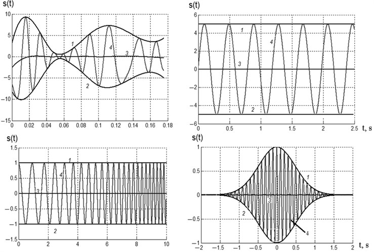
The envelopes are usually interpolated by cubic splines. Below we can find several examples of IMFs. 1 – indicates the upper envelope, 2 – indicates the lower envelope, 3 – shows the local mean and 4 is the IMF itself. As can be seen from Fig. 1 the local mean is very close to zero for all four IMFs and the number of extrema equals the number of zero-crossings or differs from it by one.
Fig. 1Examples of IMFs
EMD represents an arbitrary signal with finite energy as a collection of IMFs and a final residual (either a constant or the mean trend) [1-8]. The main idea behind the whole decomposition procedure is that at each step a new IMF, which is a detailed component highlighting high-frequency effects, is extracted. Along with this IMF, a new residual, highlighting low-frequency effects, is formed, and subsequently used for extracting the remaining IMFs. Thus, an IMF is a fast oscillating component reproducing high-frequency details, whereas a current residual is a slowly oscillating one (in comparison with an IMF), responsible for low-frequency details. Provided that a current residual has at least one maximum and one minimum, decomposition proceeds. Otherwise, the IMF extraction is terminated and a final monotonous residual is formed and the decomposition is complete.
The key role in EMD is played by the sifting process [1, 2], which is iterative and directed at extracting an IMF satisfying the two necessary conditions mentioned above. While sifting components, those which do not have properties (1) and (2) are not taken into account. The number of iterations for each IMF depends on the symmetry of a current residual and a specially designed stopping rule. When decomposition is finished, a signal may be reconstructed including all the components derived or sometimes deliberately excluding some of them from consideration (for example, if they are redundant). In general, the summation index in the reconstruction formula does not have to vary over all possible values of indices (from the first to the last) but belongs to the so-called index set . This modification is intended to preserve those IMFs which represent typical patterns of the observed signal.
2. Signal denoising
Among the main applications of EMD are signal denoising and signal detrending. They are both related to signal preprocessing because they affect all further operations with signals under study.
Signal denoising can be described the following way. The original signal contaminated with noise is This signal contains additive noise with constant variance (if the variance is not constant, we will deal with heteroscedastic noise also considered in this paper). We assume that noise power is much less than signal power , i.e. Noise distribution is Gaussian.
The original additive mixture of wanted signal and noise is:
where is the mixture of signal and noise; is wanted signal; is additive noise.
As a result of denoising we need to extract the wanted signal and find its estimate . This estimate can be written as:
where is an operator that depends on the denoising technique.
In our paper the operator is a non-linear thresholding operator [9-11] for IMF samples.
3. IMF thresholding
Thresholding is one of the most efficient techniques of signal denoising [9-11]. Thresholding helps avoid the problems that arise in other denoising techniques combined with EMD. In particular, we reduce the probability of confusing the wanted high-frequency signal and noise. Thresholding does not require us to choose the thresholds manually like in the confidence interval technique. Thresholding is based on estimating standard deviation using statistical data. The thresholding itself is not applied to all signal components, but only to several initial ones (normally, 3 or 4 IMFs) that contain noise. After denoising we perform signal reconstruction by summing the modified IMFs.
Thus, any IMF from initial IMFs is represented the following way:
where is the number of a decomposition level; is the component that corresponds to the wanted signal; is the noise component. Now we can produce a general expression for finding :
where is a non-linear operator responsible for modifying IMF samples; is the threshold affecting the denoising procedure.
The formula for finding provided above allows us to distinguish between hard and soft thresholding:
1) Hard thresholding of IMF samples:
2) Soft thresholding of IMF samples:
Hard thresholding is also called “keep or kill”. In hard thresholding an IMF sample remains the same if its absolute value exceeds the threshold and the sample is modified otherwise. The hard thresholding algorithm can be written the following way:
where is the modified component.
Soft thresholding is also called “modify or kill”. In soft thresholding, unlike hard thresholding, we do not set IMF samples equal to zero (if the absolute value of these samples is less than the threshold), but modify them using a special formula. Soft thresholding can be represented as:
where:
There are also several alternative thresholding procedures that operate between hard and soft thresholding. Fig. 2 illustrates soft and hard thresholding (Fig. 2(a) and 2(b)) and the modified thresholding.
Fig. 2Graphs for soft, hard, and modified thresholding
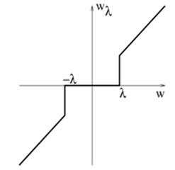
a)
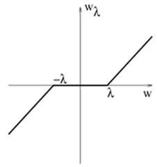
b)
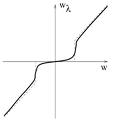
c)
Application of thresholding requires us to know the thresholds :
where is the estimation of the noise standard deviation for th IMF. It is possible to compute the standard deviation for each IMF and use different thresholds for different decomposition levels. We can also apply the universal threshold for all components (IMFs) simultaneously.
Estimation of the standard deviation can be performed the following way [9]:
This median estimate is obtained for Gaussian noise and it is stable to outliers in the original data.
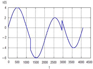
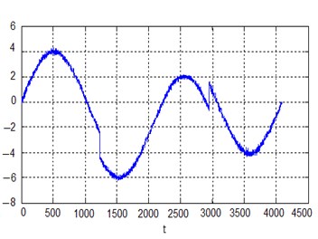
Below we can see the examples of soft and hard thresholding using the median estimate of the noise standard deviation. These examples illustrate denoising for smooth signals containing local singularities. Fig. 3(a) shows a pure sinusoidal signal with two local singularities and Fig. 3(b) the signal corrupted with white Gaussian noise (on the right) .
Fig. 3a) Pure sinusoidal signal and b) the same signal with noise N0; 0.12
a)
b)
After applying hard thresholding, which is recommended in the case of local singularities, we obtain the result shown in Fig. 4. The first five decomposition levels have been used for hard thresholding.
Fig. 4Signal after denoising using hard thresholding
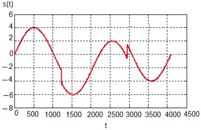
Fig. 5Denoising results for local singularities
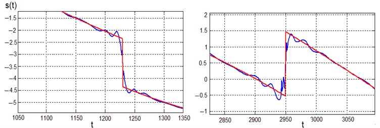
Fig. 5 shows the results of hard thresholding for local singularities. As can be seen from the figure, there are local oscillations, but their magnitude is not significant. We can conclude that the quality of signal denoising using hard thresholding is satisfactory.
4. IMF thresholding in the case of heteroscedastic noise
Depending on the variance we can distinguish between two main types of noise:
– homoscedastic noise – noise with constant variance;
– heteroscedastic noise – noise with variable variance.
The model of heteroscedastic noise can be represented as:
where , ,…,,..., are noise variances at local segments; , ,…, , ,…, , are time points where the noise model changes.
We propose signal denoising in the case of heteroscedastic and homoscedastic noise based on EMD and a classification statistics. First, we will express the connection between the original signal and IMFs extracted by EMD:
where is the original signal, is the final residual, is the th IMF, is the total number of components including the final residual ( IMFs and the final residual).
EMD is a complete decomposition, i.e. the original signal can be represented as a sum of IMFs and the final residual, which is a trend component.
Due to dyadic filter bank structure of EMD we can conclude that the 1st IMF occupies the widest frequency band (acting as a bandpass filter) in the frequency domain and the last IMF and the final residual occupy the smallest frequency band (acting as a lowpass filter). Since the original signal contains noise (heteroscedastic or homoscedastic) it can approximated by the 1st IMF:
where is the approximation of noise and .
Each IMF makes a contribution to the original signal and this contribution can be estimated by weights introduced for each IMF. Though the estimates of these weight coefficients are close to unit, they are still different from each other and later these estimates will be used for IMF classification and signal denoising:
where are weights (weight coefficients). This equation can be transformed into vector-matrix form:
where is the original signal (represented as a vector), is noise (represented as a vector), is the vector of weight coefficients, is the matrix of IMFs (each column of this matrix is an IMF including the final residual, but the 1st IMF is excluded from this matrix due to its use as noise approximation).
Using the least-squares method we can estimate the vector of weight coefficients:
We can also find the confidence interval for each weight coefficient using the confidence probability 0.95:
where , are the true value of th coefficient and its estimate, respectively, and is a fractile of -distribution.
Next, we can subject all the coefficients to a statistical significance test and use a special classification statistics:
where is a covariance matrix of IMFs calculated as , is an estimate of noise standard deviation. The standard deviation of noise can be found as a median estimate or least squares estimate. The median estimate is used more often since it is robust to outliers in the original dataset (signal):
Next, we will illustrate several examples using signals with heteroscedastic noise and the classification statistics introduced above. Consider a harmonic signal with heteroscedastic noise (Fig. 6). EMD for this signal with parabolic envelope interpolation yields 3 IMFs and the final residual. The decomposition is shown in Fig. 6 and the characteristics of IMFs are provided in Table 1.
Table 1Distribution of IMFs for a harmonic signal with heteroscedastic noise
IMF (component) | computed by least squares method | Left boundary of confidence interval | Right boundary of confidence interval | Length of confidence interval | 10-3 |
2 | 0.6733 | 0.5864 | 0.7601 | 0.1737 | 0.0128 |
3 | 0.8361 | 0.7701 | 0.9020 | 0.1320 | 0.0208 |
4 | 0.9998 | 0.9995 | 1.0001 | 0.0006 | 5.1809 |
The classification statistics for the 4th component (final residual) differs much from those for the initial IMFs and the final residual is the original monoharmonic after denoising. The plot of the denoised signal is shown in Fig. 7 and we can conclude that heteroscedastic noise has been excluded successfully.
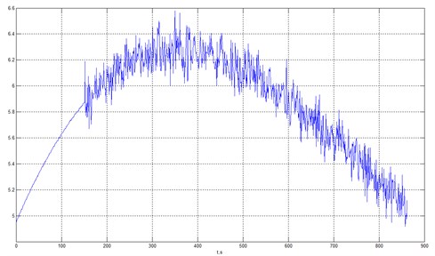
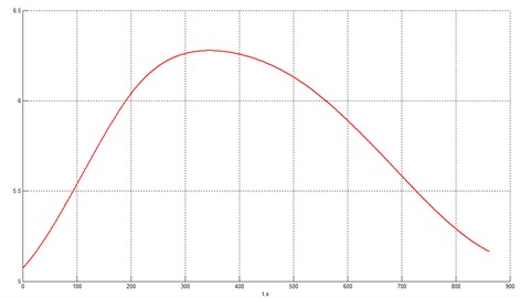
Consider another example of heteroscedastic noise combined with a smooth curve (quadratic polynomial). The original signal contaminated with noise is shown in Fig. 8.
Application of EMD yields 6 components shown in Fig. 9.
Fig. 6EMD of a harmonic signal with heteroscedastic noise
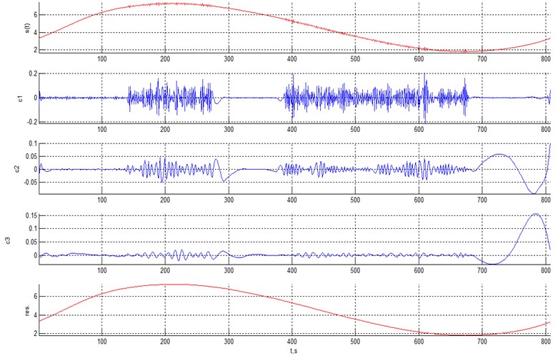
Fig. 7Harmonic signal after denoising (heteroscedastic noise)
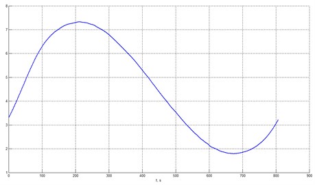
Fig. 8Smooth curve (quadratic polynomial) with heteroscedastic noise
The distribution of the extracted components is given in Table 2.
As can be seen from the Table 2, the classification statistics for the 6th IMF is different from the initial IMFs and the 6th IMF represents the original smooth curve without heteroscedastic noise. The graph is shown in Fig. 10.
Table 2Distribution of IMFs for a smooth curve with heteroscedastic noise
IMF (component) | computed by least squares method | Left boundary of confidence interval | Right boundary of confidence interval | Length of confidence interval | 10-3 |
2 | 0.9580 | 0.8964 | 1.0196 | 0.1232 | 0.0256 |
3 | 0.9598 | 0.8934 | 1.0263 | 0.1329 | 0.0238 |
4 | 0.8725 | 0.6625 | 1.0824 | 0.4199 | 0.0068 |
5 | 0.9663 | 0.7739 | 1.1587 | 0.3849 | 0.0083 |
6 | 0.9999 | 0.9992 | 1.0006 | 0.0014 | 2.3517 |
Fig. 9EMD of a smooth curve with heteroscedastic noise
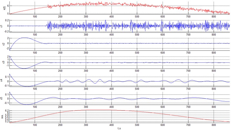
Fig. 10Smooth curve after denoising (heteroscedastic noise)
5. Engineering applications of the suggested denoising technique
The suggested denoising technique based on EMD can be used for denoising vibrational signals containing homoscedastic and heteroscedastic noise. Vibrational signal is a signal containing information about the level of vibrations of different objects. Vibrational signals often require preprocessing because it helps improve the accuracy of estimating various parameters of vibrational signals and objects.
Vibrational signals can be distorted by noise. This noise can be caused by failures of receivers and sensors responsible for signal reception. This noise in the original vibrational signal impedes full analysis of signals and therefore should be removed. In our paper we consider the analysis of signals when the whole signal is known and therefore we can apply certain techniques, like EMD, which are not suitable for real-time processing without proper modifications.
After denosing we can estimate different parameters of a vibrational signal in the time and frequency domains. Some examples of these parameters are listed below:
1) Initial time points of different processes in a vibrational signal (time domain);
2) Final time points of different processes in a vibrational signal (time domain);
3) Power spectral density of stationary vibrational processes;
4) Vibration energy in different frequency bands.
These parameters are usually very informative for real vibrational signals and characterize various objects.
6. Conclusions
In this paper we have illustrated the use of EMD for signal denoising, which is often included in the list of tasks used for signal processing. Due to adaptivity EMD has been demonstrated as an efficient tool for signal denoising for the case of homoscedastic and heteroscedastic noise. We have also discussed some applications of denosing in vibrational signal processing and analysis.
References
-
Huang N. E., Shen S. S. P. The Hilbert Transform and its Applications. World Scientific, 2005.
-
Huang N. E., et al. The empirical mode decomposition and the Hilbert spectrum for non-linear and non-stationary time series analysis. Proceedings of the Royal Society of London, Vol. 454, 1998, p. 903-995.
-
Flandrin P., Rilling G., Gonsalves P. Empirical mode decomposition as a filter bank. IEEE Signal Processing Letters, Vol. 11, Issue 2, 2004, p. 112-114.
-
Huang N. E.,Shen Z., Long S. R. A new view of nonlinear water waves: the Hilbert spectrum. Annual Review of Fluid Mechanics, Vol. 31, 1999, p. 417-457.
-
Rilling Gabriel, Flandrin Patrick, Goncalves Paulo On empirical mode decomposition and its algorithms. Proceedings of IEEE-EURASIP Workshop on Nonlinear Signal and Image Processing NSIP-03, Grabo, Italy, 2003.
-
Flandrin Patrick, Rilling Gabriel, Gonçalvés Paulo Empirical mode decomposition as a filter bank. IEEE Signal Processing Letters, Vol. 11, Issue 2, 2004, p. 12-114.
-
Okine Nii Attoh, Barner Kenneth, Bentil Daniel, Zhang Ray The empirical mode decomposition and the Hilbert-Huang transform. EURASIP Journal on Advances in Signal Processing, 2008, p. 251518.
-
Rato R. T., Ortigueira M. D., Batista A. G. On the HHT, its problems, and some solutions. Mechanical Systems and Signal Processing, Vol. 22, Issue 6, 2008, p. 1374-1394.
-
Mallat S. A Wavelet Tour of Signal Processing. Academic Press, 2008.
-
Donoho D. L., Johnstone J. M. Minimax estimation via wavelet shrinkage. Annals of Statistics, Vol. 26, Issue 3, 1998, p. 879-921.
-
Donoho D. L., Johnstone J. M. Ideal spatial adaptation by wavelet shrinkage. Biometrika, Vol. 81, Issue 3, 1994, p. 425-455.
Cited by
About this article

