Abstract
To solve the multivariable multi-step prediction problem in chaotic complex systems, this paper proposes a local Volterra model based on phase points clustering. Firstly, reconstruct the phase space of the data and calculate the similarity of the evolution trajectories. According to the similarity, the initial clustering center of the observation point is calculated and the clustering is carried out by means of K mean. We find the cluster class nearest to the prediction phase, compare the predicted phase point with the evolutionary trajectory similarity of all the observed points in the cluster, select the optimal neighboring phase point, and the optimal neighboring phase point is used for training and multi-step prediction of the multivariable local Volterra model. The proposed model method can greatly reduce the time of multi-step prediction and improve the efficiency of prediction. Finally, by experimenting with the data of Beijing PM2.5 acquired from UCI machine learning database, the experimental results show that this model method has better predictive performance.
1. Introduction
Chaotic time series prediction is an important application field and research hotspot of chaos theory [1]. In recent years, with the development of nonlinear science, multivariable chaotic time series prediction shows a greater advantage than univariate chaotic time series prediction, Multivariable chaotic time series prediction has wide application prospect in many aspects such as weather forecasting, runoff forecasting, economic forecasting, wind and electricity load forecast [2], stock forecasting [3] and target trajectory prediction. The research object of this paper is air pollutant PM 2.5. In general, air pollutant emissions are important indicators for evaluating environmental management and implementing new strategies. Fine particles (PM2.5 or PM10) contain particles no larger than 2.5 μm or 10 μm [4]. These particles are an important part of air pollution and are mainly caused by the combustion of fossil fuels and air pollutants such as NO2, CO, and SO2. High concentrations of PM2.5 can cause serious air pollution, causing a series of respiratory and pulmonary diseases, and have a serious impact on public health [5]. PM2.5 is influenced by multivariable factors such as NO2, CO, humidity, wind speed and wind direction, and has non-linear relationship with air quality and meteorological data. In order to obtain higher prediction accuracy, researchers in recent years have made a lot of researches on the methods of predicting the concentration of PM2.5, PM10 and other air pollutants [6]. For the linear prediction method, Jian et al. used the ARIMA model to study the influence of meteorological factors on ultrafine particulate matter (UFP) and PM10 concentrations under heavy traffic conditions in Hangzhou [7]. Vlachogianni et al. using multivariate linear regression model to predict the NOx and PM10 concentrations in Athens, the NO, NO2, CO and PM 2.5 concentrations were used as predictive variables [8]. The prediction models such as Arima and MLR have been widely used to predict PM concentration, but the linear method can provide reliable prediction result only when the time series data is linear or near linear, however, this kind of method still has wide application scope in the Prediction field [9]. For nonlinear predictive methods, for example, Cobourn, a nonlinear regression model is proposed to predict PM 2.5 air quality in Kentucky State Louisville metropolitan Area [10]. Artificial neural Network (ANN) model has the ability of detecting response and complex non-linear relationship between predictive factors, and can be trained by many effective training algorithms, therefore, artificial neural network model has aroused more and more attention in the field of air quality prediction [11]. For example, Pérez et al. uses the artificial neural network model to predict PM2.5 concentration and humidity by using wind speed and wind direction and PM2.5 concentration as predictive variables [12]. Fernando et al. show that the artificial neural network shows the advantages of fast calculation and high precision, can be used for the rapid development of air quality early-warning system, ANN prediction error changes according to the predicted range and different input variables. Although artificial neural network can produce better prediction results, the disadvantage of this method is that it requires a large number of training samples and results in unstable training results [13].
In recent years, with the progress and development of functional theory, Volterra filter has gained wide attention with its advantages of fast training speed, strong nonlinear approximation ability and high prediction accuracy [14]. At present, domestic and foreign scholars have conducted a series of researches on the multi-step prediction of high dimensional chaotic time series by Volterra functional technology, and its application is continuously deepening and refining. Literature [15] proposed the wind power prediction genetic algorithm-Volterra neural network (GA-VNN) model. This method combines the structural characteristics of the Volterra functional model and the BP neural network model, and uses the genetic algorithm to improve the combination model. In terms of global optimization capability, the predictive performance of wind power super short-term multi-step prediction is significantly higher than that of Volterra model and BP neural network model. However, this combination model has short prediction steps, large application limitations, and complex structures. Larger, less predictive efficiency. The above method only improves multi-step prediction performance from a single point of view, and does not fully consider the comprehensive factors such as prediction accuracy, prediction efficiency, multivariate information, and applicability. The literature [16] proposed a Volterra-based multivariate chaotic time series multi-step prediction model. This method expands the univariate Volterra filter into a multivariate, taking into account the effect of multivariate information on the performance of multi-step predictions. When the number is small, its multi-step prediction performance is better than that of the univariate Volterra model and the multivariable local polynomial model. However, because the model is based on global prediction and multi-step prediction, when the data volume is large, its multi-step prediction efficiency needs further improvement. It is one of the most efficient and common methods to predict high-dimensional chaotic complex systems through local modeling. The key to improving local multi-step prediction accuracy is to select a reasonable neighboring phase point. The current major criteria are: Distance, direction and distance comprehensive criteria, vector similarity and so on [17]. According to the theory of complex systems, the correlation information between multi-dimensional variables and observational data are all involved in the evolution of the system. The above criteria do not fully consider the association information between variables and multi-steps when selecting the optimal neighboring phase points. Comprehensive factors such as the evolutionary rule after the retrogression and the acting forces at different locations. At the same time, for the selection of the optimal neighboring phase points, the traditional local area prediction method compares the predicted phase points with all observed phase points in the phase space, and the amount of calculation is large. In particular, selecting the optimal neighboring phase point in observation points with a large amount of data has a long operation time, which greatly reduces the multi-step prediction efficiency. Currently, there is no effective solution to the related literature.
PM2.5 concentration chaotic time series data is affected by multiple variables such as temperature and wind speed in the prediction. To improve the prediction accuracy, a multi-step local model Volterra multivariable chaotic time series prediction model based on phase clustering is proposed. The experimental data was collected from UCI Machine Learning Repository’s US Embassy in Beijing within five years of weather reporting and pollution levels. Modeling the PM2.5 concentration, based on the multi-variable local Volterra multi-step prediction model, combined with the evolution law of multi-step backtracking of adjacent phase points and the influence of the correlation information between variables on the evolution trajectory of phase points, A new multivariate evolution trajectory similarity synthetical criterion is used to improve the precision of multi-step prediction of PM2.5 concentration by selecting a reasonable neighboring phase point. According to the characteristics of the similarity between observation points in phase space, the observation phase points are first clustered, and then the similarity degree is compared between the phase points and the nearest cluster phase point to select the optimal neighboring phase point. Reduce the number of calculation iterations and reduce multi-step prediction time. The idea of phase cluster analysis is used to improve the multi-step prediction efficiency of PM2.5 concentration, and ultimately achieve the purpose of comprehensively improving multi-step prediction performance of multi-variable local Volterra model. It has broad application prospect and value in air quality prediction.
2. Local Volterra multivariable chaotic time series prediction
2.1. Multivariate phase space reconstruction
The phase space reconstruction is the basis of studying and analyzing the chaotic dynamical system. According to Takens’s theorem, as long as choosing the appropriate embedding dimension, that is , the reconstruction of the phase space will have the same geometry as the original power system, and it’s equivalent to the original power system, where is the embedded dimension and is the singular attractor dimension of the chaotic system [18].
For the multi-variable phase space reconstruction technique, given the chaotic time series of dimension multivariable:
The multi-variable chaotic time series is reconstructed as follows:
where and represent the delay time and embedding dimension of the th variable, respectively, and , , and .
2.2. Multivariable local Volterra prediction model
The Volterra model of a single variable is extended to be a multivariable Volterra model [19], because the Volterra functional is very difficult to apply to the actual situation by the infinite series expansion. In general, the sum of is usually used and the second order truncation is performed. The form is as follows:
After the state is expanded, the total number of coefficients is:
The input vector of the multivariable Volterra filter is:
where is the input vector of the th variable, 1, 2, ..., , and the filter coefficient vector is:
The multivariable Volterra filter output (3) can be written as:
Multivariable Volterra filter prediction error is:
3. Select the optimal adjacent phase point
The selection of traditional adjacent phase points is mostly based on the similarity of the one-step evolution of the chaotic orbit, which lacks the consideration of the overall evolution of the system, and ignores the influence of the correlation information between variables on the evolutionary trajectory. When the prediction step is longer, the prediction trajectory and the original trajectory deviate greatly. In order to improve the learning performance of the model, avoid increasing the complexity of the model, while avoiding the influence of the relative weak phase point on the model precision, the selection of the adjacent phase point should not only select the phase points similar to the prediction point evolution trajectory in many phase points, but also control the number of adjacent points. Therefore, by defining the mutual information relative contribution rate, the multi-step evolution distance similarity and multi-step evolution direction to measure the similarity of the multivariate evolutionary trajectory, this paper proposes a selecting optimal adjacent phase points synthesis criterion.
Mutual information can better reflect the statistical dependence of variables, and mutual information can be used for multivariate correlation analysis [20]. In order to avoid the direct estimate of high dimensional probability density function, based on the estimation of adjacent mutual information [21], the relative contribution rate of the input variable to the nearest neighbor information value is used to represent the correlation information between variables. The basic method of adjacent mutual information estimation is: if represents point to its th neighbor distance, the distance between the -axis and the -axis is respectively, and the mutual information estimation of variables and is:
where is the digamma function, which is generally written as ; and are the number of data points of the conditions of and ; represents the average of all of these variables.
For multivariate, the mutual information can be extended by Eq. (10) to:
where is the dimension of the variable. Based on the relative contribution of different input variables to the overall mutual information value, the correlation between multivariate variables is analyzed. Let be the subset of input variables, means to remove a subset of variables in the set (), and is the output variable.
The relative contribution rate of the variable to the mutual information is defined as:
Criterion 1: The distance similarity between the predicted point and the phase point is as follows:
where , , , and is smaller, the closer the evolution distance of the step of the adjacent phase point is to the step evolution of . Considering the smaller phases of the backtracking step, the greater the role of the prediction point, the weighted processing of the action of the multi-step backtracking point. Define the back step distance weight vector , , and satisfy the condition: , .
The weighted treatment of the similarity of multi-step evolution distance is:
2) Criterion 2: The direction distance similarity between the predicted point and the phase point is as follows:
where , , represents the inner product of vectors, represents the distance norm of the vector, represents the absolute value, and the smaller the value of , the closer the step evolution direction of the adjacent phase point is to the step of . Define backward step weight vector , meet the condition: , take . The weighted processing of the similarity of multi-step evolution direction is:
3) Comprehensive criterion multivariate evolutionary trajectory similarity.
The evolutionary trajectory similarity between the prediction point and the phase point of the single variable is:
where , are the weight values of the distance index and the direction index, respectively, and 1, 1, 2, …, represents the number of variables. The value of is smaller, indicating that the prediction point of a single variable is similar to that of phase point . Based on the relative contribution of input variables to the mutual information value, the similarity of the single variable evolution trajectory are extended to the multivariable, and the similarity of the evolution trajectory of the predicted point and the phase point of the input variable set is as follows:
Finally, according to the multivariate evolution similarity index selected the optimal point data, carrying on the training model.
4. Adjacent points clustering analysis
For the selection of the optimal adjacent point, the traditional local prediction method is to compare the predicted phase point with the global observation point, the calculation time is longer and the prediction efficiency is lower. For this reason, based on the -means clustering algorithm, this paper proposes a new scheme based on adjacent phase point clustering analysis. Firstly, the observation phase points are analyzed by clustering, and then the predicted phase points are compared with the nearest cluster phase points, and the optimal adjacent phase points are selected to reduce the prediction time.
Due to the complexity of multi-variable observation point, the cluster with different sizes and densities may be formed. The -means algorithm is not very good for the data clustering of heterogeneous distribution. In order to prevent the density of the cluster from being too high and influence the prediction accuracy, the weighted processing of the sum of the errors in the cluster is carried out, and the criterion function of the clustering is defined as:
where is the number of cluster centers, represents the total number of elements of the data set, stands for category , represents the number of elements in the th class, represents the clustering center vector of class , and represents the element vector belonging to class .
The clustering analysis of adjacent phase points takes the predicted phase points as the reference standard of the evolutionary trajectory similarity, and then clustering the evolutionary trajectory similarity of all the observation points. By the Eq. (17), the similarity vector of the multivariate evolution trajectory is defined as:
By Eq. (18), the similarity value of multi-variable evolution trajectory of observation phase points is calculated, which is ranked as in ascending order and (integer) as the interval. In turn, the evolution path similarity vector of corresponding phase point is selected as the initial cluster center, and the initial cluster center can be dispersed as far as possible to close to the final clustering center and reduce the time of clustering.
The update formula of clustering center is:
Based on the relative contribution rate of input variables to the mutual information value, by Eq. (12), the vector of the multi-variable mutual information contribution rate is:
Define a new operator symbol:
According to the multidimensional evolutionary trajectory similarity clustering feature of the phase point, from Eqs. (20-23), (19) can be expressed as:
5. The implementation step of multivariable multi-step prediction
For the multi-step prediction problem of high-dimensional chaotic system, a lot of practice shows that most nonlinear dynamical systems can be characterized by Volterra series [22-24], so we can construct multi-step chaotic time series multi-step prediction model with Volterra series expansion. Therefore, in order to make the multivariate adjacent phase points selection more reasonable and more efficient, this paper proposes a local Volterra multivariable chaotic time series multi-step prediction based on phase points clustering. The concrete steps are as follows:
Selection of input variables and multivariate phase space reconstruction;
Taking the predicted phase points as the reference standard of evolution trajectory similarity, the multi variable trajectory similarity vector of all observation points is calculated, which is used as the data set to be clustered, and determined the number of clustering centers ;
The prediction phase point is used as the reference standard for the similarity of evolutionary trajectory. In order to form clusters, we calculate the similarity value of multivariate evolutionary trajectory of all the observed phase points, and take the value of ascending arrangement and equal interval, then select corresponding phase point's evolution trajectory similarity vector as the initial cluster center.
By redistributing the phase point, the value of the criterion function is minimized, and new clusters are formed and the cluster centers are updated.
Cycle step 4, until the cluster centers are not changed, clustering is completed;
The evolution trajectory similarity vector of the predicted phase point is calculated, and calculate the distance to each cluster center , choose the nearest cluster, and the prediction phase point is compared with the similarity of the evolution trajectory of all the observation points in the cluster, and the d optimal adjacent phase points are selected from this.
The optimal adjacent phase points are used to train the multivariable Volterra model. and the multivariable coefficient vector is obtained, and the input vector is generated by the prediction phase point, and the one-step prediction value is given.
The predictive value is entered into the observational data, then iterated, and the function of multi-step prediction is finally realized.
The multi-step prediction performance of this model depends on the rationality and efficiency of the selection of the optimal adjacent phase points.
The realization step of multi-step prediction. According to the local Volterra prediction model proposed in this paper, we can get the first step prediction value. In the second step prediction, the first step prediction value is added as the known value to the historical data to calculate the second step Prediction value, when calculating the prediction value of the third step, the prediction value of the second step of the first step is added as the known value to the historical data to calculate the prediction value of the third step. According to this method, according to the model Continuous iteration for multi-step prediction.
6. Simulation and result analysis
6.1. Experimental data
Experimental Data from the UCI machine learning database for the five-year weather report and pollution levels of the U.S. embassy in Beijing. , , three components as input variables, where , , , respectively, PM2.5 concentration, temperature, wind speed. component as a predictor of the proposed model to verify. Each component received 5050 data points, of which the first 5000 data points as training data, the remaining 50 data points as the test data, and the data normalized. By means of saturation correlation dimension method and mutual information method, the embedded dimension of input variables is determined as 3, and the delay time is 12 respectively. The weight values u1 and u2 of the distance and direction in the comprehensive criterion are respectively 0.58 and 0.42. The relative contribution rates of the and variables to the mutual information value are 32.5 % and 27.6 % respectively. Experimental hardware conditions: Inter (R) Core (TM) i7-6700 CPU@3.40GHz, 16GB memory. The software environment: MATLAB2016a.
6.2. The judgment of chaotic characteristics
In this paper, the chaotic characteristics of PM2.5 concentration, temperature and wind speed are identified by the saturation correlation dimension method. Crassberger and Procaccia [25, 26] proposed the correlation dimension method to investigate the chaotic characteristics of time series. For random sequences, the correlation dimension increases with the increase of embedding dimension, and does not reach saturation. For the chaotic sequence, correlation dimension tends to saturation gradually along with the increase of the embedding dimension. Therefore, we can distinguish the chaotic sequence from the random sequence according to whether the correlation dimension is saturated or not.
Consider the vector set near the attractor , the associated integral is defined as the number of points that are less than r for any given r, and the ratio of the number of points to all possible points, that is:
where:
when , for any small , we can follow the law of the exponential power change of , which is , and we can calculate by the derivative of with . In this paper, the G-P algorithm [27] is used to calculate the saturation correlation dimension of the time series. Figs. 1-3 respectively show the and curves of PM2.5, temperature and wind speed time series, where is the correlation function and is the radius.
Fig. 1PM2.5 time series lnC(r)-lnr graph
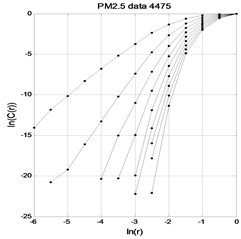
Fig. 2temperature time series lnC(r)-lnr graph
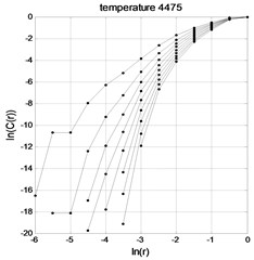
Fig. 3wind time series lnC(r)-lnr graph
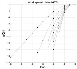
As shown in Figs. 1-3, the and curves gradually become parallel with the embedding dimension increasing, that is, the correlation dimension gradually reaches saturation. According to Eq. (8), the attractor dimension of PM2.5 in temperature and wind speed time series is respectively 2.3576, 0.7144 and 1.2835. The attractor dimension is fractional Form, indicating that there are chaos characteristics in time series of PM2.5, temperature and wind speed.
6.3. Select the number of the optimal adjacent phase point
In order to verify the influence of the number of the nearest neighbor points on the prediction accuracy, the optimal adjacent points with different numbers are selected for comparison experiment. Using the comprehensive criterion of multivariate evolution trajectory and prediction model presented in this paper, and take the root mean square error (RMSE) as the evaluation criterion as shown in Eq. (26), where represents the observation value, represents the true value, represents the number of data points, the comprehensive criterion of multivariate evolution trajectory and prediction model proposed in this paper are used. The comparison results are shown in Table 1:
As can be seen from Table 1, using the comprehensive criterion of multivariate evolution trajectory and prediction model presented in this paper, in the one-step, five-step and ten-step prediction, when the number of the nearest neighbor points increases from 2 to 12, the prediction error decreases gradually. When the number of the nearest neighbor points is more than 12, The error increases gradually, so when the number of nearest neighbor points is 12, the overall prediction error is the smallest.
Table 1The effect of adopting different number of nearest neighbor points on multi-step prediction performance
The optimal number of adjacent points | One step prediction error | Five-step prediction error | Ten-step prediction error |
2 | 6.425×10⁻² | 4.417×10⁻¹ | 7.836×10⁻¹ |
4 | 3.794×10⁻² | 2.109×10⁻¹ | 5.791×10⁻¹ |
6 | 1.681×10⁻² | 1.365×10⁻¹ | 4.217×10⁻¹ |
8 | 7.175×10⁻³ | 8.712×10⁻² | 1.054×10⁻¹ |
10 | 4.103×10⁻³ | 3.538×10⁻² | 3.319×10⁻² |
12 | 2.394×10⁻³ | 1.627×10⁻² | 2.476×10⁻² |
14 | 5.217×10⁻³ | 5.194×10⁻² | 6.245×10⁻² |
16 | 3.106×10⁻² | 1.328×10⁻¹ | 2.207×10⁻¹ |
18 | 1.329×10⁻² | 3.619×10⁻¹ | 5.758×10⁻¹ |
6.4. Verify the validity of the comprehensive criteria
In order to validate the validity of the similarity criterion of evolutionary trajectories proposed in this paper, comparison experiments with other commonly used criteria are carried out. The number of the nearest neighbor points is set as 12. The prediction model uses the model proposed in this paper and the root mean square error (RMSE) as the evaluation criterion as shown in Eq. (26), the results shown in Table 2.
Table 2The effect of different criteria on multi-step prediction performance
Criterion | One step prediction | Five-step prediction | Ten-step prediction |
Euclidean criterion | 5.08×10⁻² | 8.74×10⁻² | 6.65×10⁻¹ |
Comprehensive criterion of direction and distance | 7.15×10⁻³ | 4.73×10⁻² | 2.26×10⁻¹ |
Vector similarity | 9.53×10⁻² | 6.63×10⁻² | 5.94×10⁻¹ |
The comprehensive criteria proposed in this paper | 2.25×10⁻³ | 1.85×10⁻² | 9.71×10⁻² |
From Table 2, it can be seen that the prediction error of the optimal adjacent phase point is large and the prediction performance is poor according to Euclidean distance in one step, five steps and ten steps prediction. Although the prediction results obtained by using the vector similarity, direction and distance criterion to select the optimal adjacent phase point are improved, the multi-step prediction accuracy of both is lower than that of the comprehensive criterion presented in this paper. It is clear that the comprehensive criterion proposed in this paper can select more reasonable adjacent points to improve the multi-step prediction accuracy of the model.
6.5. Select the number of cluster centers
The 5000 groups of training data produced by the Lorenz model for multivariate phase space reconstruction, and a total of 4976 phase points are generated, the 4976th phase point as the prediction phase point, the first 4975 phase points as the observation phase point, and the prediction phase point as the reference standard of the multivariate evolution trajectory similarity, The multivariate evolutionary trajectory similarity vectors of all the observed phase points are calculated as data sets for clustering. The evolution trajectory similarity vector of the first 4975 observation points is shown in Table 3.
In order to study the influence of the number of clustering centers on the prediction time and precision, the root mean square error of the ten-step prediction is used as the evaluation criterion, and the time of consumption is calculated by the 50-step prediction range. The prediction model uses the model proposed in this paper. the experimental results are shown in Table 4.
Table 3The evolution trajectory similarity vector of the observation point
X component | Y component | Z component |
0.0574 | 0.0613 | 0.2837 |
0.0385 | 0.0572 | 0.2635 |
0.0176 | 0.0245 | 0.1439 |
⋅⋅⋅ | ⋅⋅⋅ | ⋅⋅⋅ |
0.0016 | 0.0047 | 0.0075 |
Table 4The influence of the number of clustering centers on predicting time and accuracy
Number of cluster centers | Prediction error | Total time-consuming/s |
2 | 4.123×10⁻¹ | 7.153 |
4 | 1.734×10⁻¹ | 5.306 |
6 | 5.167×10⁻² | 2.527 |
8 | 8.109×10⁻³ | 1.128 |
10 | 3.285×10⁻² | 2.637 |
12 | 6.497×10⁻² | 4.417 |
14 | 8.536×10⁻² | 6.973 |
As can be seen from Table 4, with the increasing number of clustering centers, the root mean square error of the ten-step prediction decreases first and then increases, and the total time-consuming of 50 steps is reduced and finally stabilizes at about 1.128 seconds. When the number of cluster centers is 8, the multi-variable evolution path similarity vector of 4976 observation phase points is clustered, and the projection of the X and Y direction is shown in Fig. 4. The clustering center and phase point distribution are shown in Table 5.
Due to the complexity and uncertainty of the multivariate evolutionary trajectory similarity vector of the observation phase points, the uneven distribution of the data sets may lead to the formation of clusters with different sizes and densities. It is shown from Fig. 4 and Table 5 that the -means algorithm clustering with weighted processing avoids the high density of elements in the cluster, makes the clustering result relatively balanced, and greatly reduces the effect on the multi-step prediction precision of the model.
Fig. 4The XY direction projection of the adjacent phase clustering
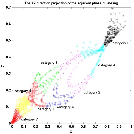
Table 5Distribution of cluster centers and phase points
Clustering center | X component | Y component | Z component | Number of phase points |
1 | 0.1909 | 0.1626 | 0.3952 | 601 |
2 | 0.8377 | 0.5395 | 0.0271 | 576 |
3 | 0.5249 | 0.3048 | 0.2138 | 1398 |
4 | 0.0976 | 0.4185 | 0.5216 | 421 |
5 | 0.0976 | 0.1096 | 0.1646 | 763 |
6 | 0.3931 | 0.1464 | 0.2385 | 453 |
7 | 0.0262 | 0.0310 | 0.0602 | 354 |
8 | 0.2909 | 0.2666 | 0.6347 | 409 |
6.6. Multi-step prediction performance comparison of each model
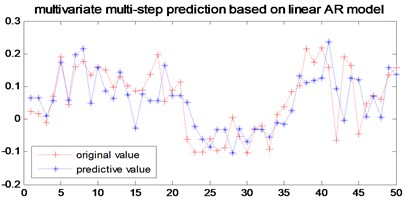
6.6.1. The local multivariable linear autoregressive model
The AR model is a commonly used time series prediction model, which has a relationship between variables of time series, and the current variable can be represented by the previous time [28, 29]. The local multivariable linear autoregressive model function can be written as:
where , , 1, …, is the fitting parameter. Combined with the evolutionary trajectory comprehensive criterion, the parameters are estimated by the least square method to calculate the predicted value.
6.6.2. The local multivariable least learning machine (ELM) prediction model
For a multivariable time series training set:
with samples, where is the input variable andis the output variable, the objective function of ELM [30] is: , , . Where is the output vector of the hidden layer; is the number of hidden nodes, is the input weight of the th hidden node; is the deviation of the th hidden node; is the output weight of the hidden layer; And for the th hidden node excitation function. According to the Lagrange multiplier method and KKT optimal conditions, we have: :
So as to obtain the prediction model .
6.6.3. The local multivariable RBF neural network multi-step prediction model
In the RBF neural network structure as shown in Fig. 5, the input vector of the network is the transpose of the input of m-dimensional vector , then the number of network input layer nodes is . Let the nodes of the hidden layer of the network have radial basis vectors and as Gauss basis functions [31]:
In this hidden layer, the center vector of Gaussian basis function of the th node is: , 1, 2, …,. The same dimensionality of and can determine the quality of the network to a large extent. Let the base width vector of hidden layer node of network be: . Where is the Gaussian basis function radius of node , the size of which determines the complexity of the network, and the appropriate value can be selected through experiments and error information; is the vector norm, which is generally the Euclidean norm.
The weight vector from the hidden layer to the output layer is:
The output function of the network is:
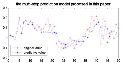
In order to verify the superiority of the proposed model algorithm, the experimental performance is compared with the multi-variable local linear AR model, multivariable local RBF neural network multi-step prediction and multivariable ELM multi-step prediction model. The experimental results are shown in Figs. 6-9.
Fig. 5RBF network structure
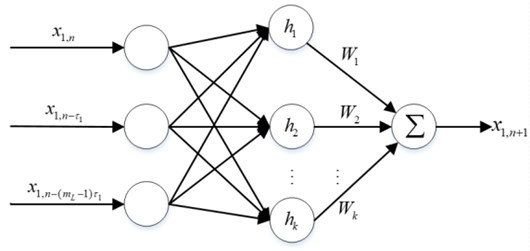
Fig. 6The multi-step prediction model proposed in this paper
a)
b)
Fig. 7multi-step prediction of local linear AR model
a)
b)
Fig. 8Multi-step prediction of local RBF model model
a)
b)
Fig. 9Multi-step prediction of local ELM model
a)
b)
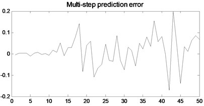
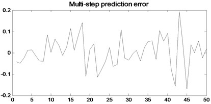
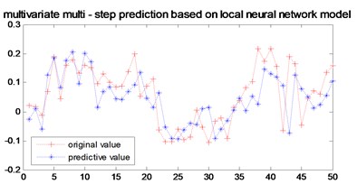
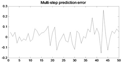
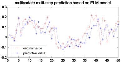
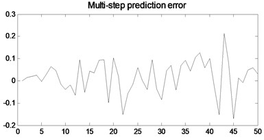
In order to verify the multi-step prediction performance of the proposed model, compared with other multi-step prediction models, the effective step size of multi-step prediction is 50 steps, as shown in Figs. 6- 9. It can be seen from Fig. 6 that the prediction accuracy of the model proposed in the previous 12 steps is very high. Although the predicted trajectory deviates from the original trajectory after 12 steps, the deviation is relatively small, indicating that this model predicts a longer prediction step Long and small prediction error. As can be seen from Fig. 7, the multivariate local linear AR model has only 4 steps for multi-step prediction. After 4 steps, the predicted trajectory deviates from the original trajectory, the prediction error fluctuates greatly, and the prediction effect is not good. As can be seen from Fig. 8 and Fig. 9, the multivariable local RBF neural network model and Multivariable Local Least Learning Machine (ELM) model have five-step and seven-step effective prediction steps. Although the prediction error is small in the effective step, the same deviation from the predicted trajectory also limits the effective step of the prediction and the prediction error is larger.
In order to verify the high efficiency of the model, the root mean square error is used as the evaluation criterion, as shown in Eq. (26), to estimate the time consumption of the 50 step prediction step. The prediction error and total time-consuming of each model are shown in Table 6. It can be seen from Table 6 that the total time-consuming forecast for multi-step prediction is only 0.835 s, which greatly improves the prediction efficiency. In summary, the local Volterra multivariable chaotic time series multi-step prediction based on phase point clustering proposed in this paper has better multi-step prediction performance.
Table 6Predictive errors and total time-consuming comparisons for each model
Multi-step prediction model | One step prediction error | Ten steps prediction error | Total time-consuming / s |
Multivariate local linear AR model | 6.317×10⁻² | 8.165×10⁻¹ | 3.725 |
Multivariable local RBF model | 2.054×10⁻² | 5.483×10⁻¹ | 9.043 |
Multivariate local ELM model | 8.523×10⁻² | 2.692×10⁻¹ | 5.416 |
The model presented in this paper | 4.564×10⁻³ | 8.627×10⁻² | 0.835 |
6.6.4. Cram’er-Rao lower bound performance evaluation
Cram’er-Rao Lower Bound (CRLB) determines a lower bound for the variance of any unbiased estimator, and the estimate for reaching this lower bound is called the minimum variance unbiased (MVU) estimator [32]. Let be the parameter to be estimated, estimate it from the observed value , they satisfy probability density function , the lower bound of the variance of any unbiased estimate is the reciprocal of Fisher’s information:
The Fisher information is defined as:
If and only if:
The unbiased estimate for all to reach the lower bound can be calculated as , which is the MVU estimator and the minimum variance is .
We use the parameters of the multivariate Volterra model as an estimator, and use CRLB to evaluate the performance of the prediction result. The time series is . For multivariate estimated parameter , its probability density function is , which satisfies two regularization conditions [33]. The Fisher information matrix is an matrix.
is defined as:
Let be an estimate of a parameter vector, , and remember that its expected vector is . The Cramer-Rao lower bound holds that the covariance matrix of satisfies:
where means that is a positive semidefinite matrix; is a Jacobian matrix whose th element is .
Fig. 10Plot of CRLB performance evaluation
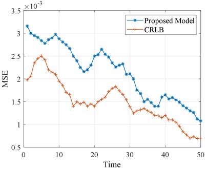
In order to better illustrate the effectiveness of the proposed algorithm, CRLB is used to estimate the lower bound of the MSE of the predicted value in a one-step prediction. Fig. 10. shows the MSE of the lower limit assessment of CRLB. The method presented in this paper also clearly shows that MSE has the same trend as CRLB and can track CRLB’s MSE well, which verifies the effectiveness and superiority of the proposed method.
7. Conclusions
Studies have shown that PM2.5 is strongly linked to other health problems such as respiratory diseases and heart and lung diseases. Protecting the environment to protect humans from air pollution, developing effective and reliable PM2.5 prediction models, and assisting environmental management departments in formulating effective environmental protection measures are urgent and indispensable requirements. PM2.5 concentration chaotic time series data is influenced by multiple variables such as temperature and wind speed in prediction, and in order to improve the prediction accuracy, a multi-step local Volterra multivariable chaotic time series prediction model based on phase clustering is proposed. Through reasonable selection of forecasting model input variables, and combining with clustering phase points, effectively solve the traditional local prediction model selection in the adjacent point problems of unreasonable and time-consuming long, and the proposed model has greatly increased the multi-step prediction step length and precision effectively, reduce the error of cumulative effect, and greatly reduce the multi-step prediction time, has broad application prospects and value in air quality forecast.
References
-
Giona M., Lentini F., Cimagalli V. Functional reconstruction and local prediction of chaotic time series. Physical Review A, Vol. 94, Issue 44, 1991, p. 3496-3502.
-
Zhou Lin, Li Furong, Tong Xing Active network management considering wind and load forecasting error. IEEE Transactions on Smart Grid, Vol. 8, Issue 6, 2017, p. 2694-2701.
-
Liu H., Huang D., Wang Y. Chaotic dynamics analysis and forecast of stock time series. International Symposium on Computer Science and Society, 2011, p. 75-78.
-
Zhou Q., Jiang H., Wang J., et al. A hybrid model for PM 2.5, forecasting based on ensemble empirical mode decomposition and a general regression neural network. Science of the Total Environment, Vol. 496, Issue 2, 2014, p. 264-274.
-
Qiu H., Yu I., Wang X., Tian L., Tse L. A., Wong T. W. Differential effects of fine and coarse particles on daily emergency cardiovascular hospitalizations in Hong Kong. Atmospheric Environment, Vol. 64, 2013, p. 296-302.
-
Pope C. A., Dockery D. W. Health effects of fine particulate air pollution: lines that connect. Journal of the Air and Waste Management Association, Vol. 56, 2006, p. 709-742.
-
Jian L., Zhao Y., Zhu Y. P., Zhang M. B., Bertolatti D. An application of ARIMA model to predict submicron particle concentrations from meteorological factors at a busy roadside in Hangzhou, China Science of the Total Environment, Vol. 426, 2012, p. 336-345.
-
Vlachogianni A., Kassomenos P., Karppinen A., Karakitsios S., Kukkonen J. Evaluation of a multiple regression model for the forecasting of the concentrations of NOx and PM 10 in Athens and Helsinki. Science of the Total Environment, Vol. 409, 2011, p. 1559-1571.
-
Thoma, Jacko R. B. Model for forecasting expressway fine particulate matter and carbon monoxide concentration: application of regression and neural network models. Journal of the Air and Waste Management Association, Vol. 57, 2007, p. 480-488.
-
Cobourn W. G. An enhanced PM 2.5 air quality forecast model based on nonlinear regression and back-trajectory concentrations. Atmospheric Environment, Vol. 44, 2010, p. 3015-3023.
-
Voukantsis D., Karatzas K., Kukkonen J., Rasanen T., Karppinen A., Kolehmainen M. Intercomparison of air quality data using principal component analysis, and forecasting of PM 10 and PM2.5 concentrations using artificial neural networks, in Thessaloniki and Helsinki. Science of the Total Environment Environ, Vol. 409, 2011, p. 1266-1276.
-
Pérez P., Trier A., Reyes J. Prediction of PM 2.5 concentrations several hours in advance using neural networks in Santiago, Chile. Atmospheric Environment, Vol. 34, 2000, p. 1189-1196.
-
Fernando H. J., Mammarella M. C., Grandoni G., Fedele P., Di Marco R., Dimitrova R., et al. Forecasting PM10 in metropolitan areas: efficacy of neural networks. Environmental Pollution, Vol. 163, 2012, p. 62-67.
-
Li Yanling, Zhang Yunpeng, Wang Jing, et al. The Volterra adaptive prediction method based on matrix decomposition. Journal of Interdisciplinary Mathematics, Vol. 19, Issue 2, 2016, p. 363-377.
-
Jiang Y., Zhang B., Xing F., et al. Super-short-term multi-step prediction of wind power based on GA-VNN model of chaotic time series. Power System Technology, Vol. 39, Issue 8, 2015, p. 2160-2166.
-
Wei B. L., Luo X. S., Wang B. H., et al. A method based on the third-order Volterra filter for adaptive predictions of chaotic time series. Acta Physica Sinica, Vol. 51, Issue 10, 2002, p. 2205-2210.
-
Zhang Xuguang, Ouyang, Zhang Xufeng Small scale crowd behavior classification by Euclidean distance variation-weighted network. Multimedia Tools and Applications, Vol. 75, Issue 19, 2016, p. 11945-11960.
-
Guo Yina, Liu Qijia, Wang Anhong, et al. Optimized phase-space reconstruction for accurate musical-instrument signal classification. Multimedia Tools and Applications, Vol. 76, Issue 20, 2017, p. 20719-20737.
-
Lei M., Meng G. The influence of noise on nonlinear time series detection based on Volterra-Wiener-Korenberg model. Chaos Solitons and Fractals, Vol. 36, Issue 2, 2008, p. 512-516.
-
Pascoal C., Oliveira M. R., Pacheco A., et al. Theoretical evaluation of feature selection methods based on mutual information. Neurocomputing, Vol. 226, 2016, p. 168-181.
-
Horányi A., Cardinali C., Centurioni L. The global numerical weather prediction impact of mean‐sea‐level pressure observations from drifting buoys. Quarterly Journal of the Royal Meteorological Society, Vol. 143, Issue 703, 2017, p. 974-985.
-
Guo Y., Guo L. Z., Billings S. A., et al. Volterra series approximation of a class of nonlinear dynamical systems using the Adomian decomposition method. Nonlinear Dynamics, Vol. 74, Issues 1-2, 2013, p. 359-371.
-
Carassale L., Kareem A. Modeling nonlinear systems by Volterra series. Journal of Engineering Mechanics, Vol. 136, Issue 6, 2010, p. 801-818.
-
Mirri D., Luculano G., Filicori F., et al. A modified Volterra series approach for nonlinear dynamic systems modeling. IEEE Transactions on Circuits and Systems I Fundamental Theory and Applications, Vol. 49, Issue 8, 2002, p. 1118-1128.
-
Grassberger P., Procaccia I. Dimensions and entropies of strange attractors from a fluctuating dynamics approach. Physica D Nonlinear Phenomena, Vol. 13, Issue 1, 1984, p. 34-54.
-
Grassberger P., Procaccia I. Measuring the strangeness of strange attractors. Physica D Nonlinear Phenomena, Vol. 9, Issue 1, 1983, p. 189-208.
-
Harikrishnan K. P., Misra R., Ambika G. Revisiting the box counting algorithm for the correlation dimension analysis of hyperchaotic time series. Communications in Nonlinear Science and Numerical Simulation, Vol. 17, Issue 1, 2012, p. 263-276.
-
Duan W. Y., Huang L. M., Han Y., et al. A hybrid AR-EMD-SVR model for the short-term prediction of nonlinear and non-stationary ship motion. Journal of Zhejiang University Science A, Vol. 16, Issue 7, 2015, p. 562-576.
-
Duan W. Y., Han Y., Huang L. M., et al. A hybrid EMD-SVR model for the short-term prediction of significant wave height. Ocean Engineering, Vol. 124, 2016, p. 54-73.
-
Kumar N. K., Savitha R., Mamun A. A. Ocean wave height prediction using ensemble of extreme learning machine. Neurocomputing, Vol. 277, 2018, p. 12-20.
-
Qiao J., Meng X., Li W. An incremental neuronal-activity-based RBF neural network for nonlinear system modeling. Neurocomputing, Vol. 302, 2018, p. 1-11.
-
Zuo L., Niu R., Varshney P. K. Conditional Posterior Cramér-Rao lower bounds for nonlinear recursive filtering. International Conference on Information Fusion, 2009, p. 1528-1535.
-
Mohammadi A., Asif A. Decentralized conditional posterior Cramér-Rao lower bound for nonlinear distributed estimation. IEEE Signal Processing Letters, Vol. 20, Issue 2, 2013, p. 165-168.
About this article

The work in this paper was supported by the National Natural Science Foundation of China under Grant No. (61001174); Tianjin Science and Technology Support and Tianjin Natural Science Foundation of China under Grant No. (13JCYBJC17700).
