Abstract
The objective in this work is to assess fatigue damages on local components of a semi-submersible platform under combined actions of wind and wave loads in time domain. Some improvements are provided in the present study to improve the efficiency and accuracy of the whole evaluating process. Firstly, a combined wind and wave relationship as well as an innovative mixture simulation method are used to generate time series of random wind and waves. Moreover, an m-block division method is proposed to compress the number of the whole short-term sea states in the wind-wave scatter diagram. Then, with an improved multiple interpolation sub-model method, the structural stress responses of the local structural components are calculated as is in the whole model analysis. Finally, a modified rain-flow counting method is provided and validated to count the stress cycles efficiently and accurately. Thus, the short- and long-term fatigue damages are computed based on the S-N curve approach and the cumulative fatigue damage rule. In relative agreement with the numerical results by the traditional time-domain method and existing experimental data, these proposed improved methods are demonstrated to be applicable and efficient methods for fatigue damage analyses. All the fatigue damages on local components satisfy the specification requirements and the minimum value appears under the up wind-wave state, which is the proper working condition for a semi-submersible platform.
1. Introduction
A semi-submersible offshore platform is utilized for the explorations and productions of offshore energy resources in more hostile and deeper ocean environments, under which circumstances the highly flexible platform is very sensitive to dynamics, such as wind, waves, currents and earthquakes [1]. Generally, structural fatigue damage occurs due to the long-term high stress concentrations. Therefore, in view of the uncertain cyclic loadings in the sea and ocean environment, fatigue becomes one important phenomenon that causes damages and failure around the weld toe on offshore structural member connections [2-5]. In consideration of the long-term structural integrity of such a complex offshore platform under the severe environmental conditions, it should be more important to accurately analyze and predict fatigue damage accumulations and consequent fatigue failure of some key local components in a proper way for a safe and reliable operation of a semi-submersible offshore platform [6, 7].
In general, waves and wind play a major role in fatigue damage accumulations due to their continuity in time and in sequence, as being tiny, moderate, and sometimes catastrophic. They produce stochastic fluctuating stress responses in offshore structural responses [8]. Generating the fluctuating wind and wave loads with a certain relationship in the present study consists of two parts: a combined relationship between wind and waves and a proper numerical simulation method. Firstly, differing from the waves-only case, a combined wind and waves case should be taken from a scatter block with three variables (i.e. wind speed, significant wave height and wave period) [9]. In the present study, a combined wind and waves relationship, based on the energy transferring relationship between wind and water surface, is explored to provide the corresponding wind speed, wave height and period according to the previous studies and the mechanism wind generating waves [10-13]. Secondly, provided that random wind and waves are a stationary Gaussian process, the combined wind and waves can be described by the power spectral density function (PSDF) [14]. Therefore, many numerical simulation methods are used to simulate the time series of the fluctuating wind and wave loads, such as the two classical approaches, the weighted amplitude wave superposition (WAWS) method [15] and auto-regression (AR) method [16, 17]. Integrating the respective advantages of WAWS and AR methods, a mixture simulation (MS) method is applied to the present study with the aid of the wavelet method, whose efficiency and accuracy has been validated in our previous work [13, 14]. Thus, a joint application of a proposed combined wind and waves relationship and an innovative proposed MS method can simulate the fluctuating wind and waves.
Fatigue is defined as a process of damage accumulation under fluctuating stress histories, which eventually results in failure. Nonetheless, the maximum working stress usually remains below the ultimate elastic limit [18]. Three fatigue damage evaluating methods are widely used to explore and determine whether the offshore structures are in a safe and reliable working condition: deterministic analysis method, frequency-domain analysis method (FDA method, i.e. spectral-based analysis method) and time-domain analysis (TDA) method [9, 19-21]. However, there are some limitations in the first two methods: the deterministic analysis method only considers the Design Wave, which leads to lower calculation accuracy compared to practical results; the spectral-based analysis method, as a widely-used method, only calculates stress with the narrow-band Gaussian random process, due to the limitation of the linear assumption [21]. Thus, as a relatively accurate method, the TDA method is adopted and improved in the present study, which generally requires the following three parts: structural dynamic response analysis [14, 22], S-N curve approach and cumulative fatigue damage rule [20, 23-25], rain-flow counting method [26, 27]. However, to improve the efficiency and accuracy of the TDA method further, an improved TDA (ITDA) method is provided in the present work and the improvements include three aspects. Firstly, considering that short-term stress response and fatigue damage calculations in every sea state should be carried out in TDA method, an -block division method is merged into TDA method to weaken the disadvantages of huge calculating load and long computing time as much as possible. Then, an improved multiple interpolation sub-model (IMISM) method together with the above-mentioned methods are used to evaluate the stress responses of local components of the semi-submersible platform [8, 21]. Finally, a modified rain-flow counting method is proposed to count the stress cycles more efficiently with no accuracy loss according to the previous study [6]. Thus, these three sub-methods in the ITDA method are applied and investigated in the present work to analyze the fatigue damages of local components of a semi-submersible platform.
The objective in the present study is to generate the wind and wave loads accurately and efficiently and propose an improved TDA (ITDA) method to better predict the fatigue damage of local components of the offshore structures. The paper is organized as follows: an ITDA method for fatigue damage analysis is proposed and the complete computational procedure for fatigue damage analysis is summarized in Section 2. The whole and local model of a semi-submersible platform in numerical simulation is presented in Section 3. Methods for generating wind and waves are provided in Section 4. Validation tests and numerical investigations are performed in Section 5.
2. Fatigue damage analysis methods in time domain
Conducting a complete fatigue damage analysis by an ITDA method generally requires the following five aspects: S-N curve approach, cumulative fatigue damage rule, rain-flow counting method, generating time histories of wind and waves and constructing and analyzing the structural model. The first three parts are introduced in this section. Due to their importance in the present study, the last two parts are presented in detail as separate sections in Sections 3 and 4, respectively. In this section, a modified rain-flow counting method is proposed to improve numerical efficiency with no accuracy lost.
2.1. S-N curve approach and cumulative fatigue damage rule
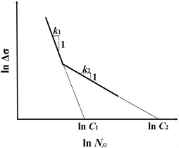
In the ITDA method, stress cycles are known as stress reversals in temporal history when fatigue damage occurs [20]. Based on a series of experimental fatigue tests, the S-N curve approach is commonly used in practice and well described in Recommended Practices and Guide for fatigue design of offshore structures [7, 23, 24]. For a better curve fitting to the fatigue test data, a multi-segmented S-N line approach sketched in Fig. 1(a) is applied in the present study [7, 18, 28], which is defined as follows:
where each segment has its own fatigue constants, and . In this model, there is consistent one-to-one match between the fatigue life and the hot-spot stress range with the constant amplitude . In practice, is determined by the nominal stress range and the stress concentration factor [29], which can be estimated from finite element analysis [18].
Fig. 1a) A sketch of a multi-segmented S-N model, b) a sketch of different applied stress cycles and corresponding fatigue lives
a)
b)
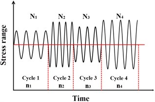
Furthermore, having defined a relation between and as presented above, the Palmgren-Miner’ rule [25, 30] is commonly applied to predict the cumulative fatigue damage under different stress ranges in practice. It is implemented in design codes [23, 24] and also conforms to the linear fatigue damage accumulation as in Eq. (1). As is sketched in Fig. 1(b), it can be described by:
In which is the total number of stress cycles applied, is the number of constant amplitude stress cycles with the stress range in Cycle , is the number of stress cycles before failure with the stress range in Cycle , and is the cumulative damage ratio in the lifetime. It is generally assumed that the fatigue failure occurs when exceeds unity (i.e. 1).
2.2. A modified rain-flow counting (MRFC) method
Developed by Matsuishi and Endo [26], the rain-flow counting (RFC) method is utilized to count the stress cycles and ranges in the random stress-time histories [20, 27, 31], whose basic principle is briefly concluded in the first subsection. Then, a MRFC method is proposed to improve the counting efficiency with less accuracy lost, whose detailed improvements is presented in the next subsection.
2.2.1. The classical RFC method (RFC method)
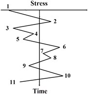
To simulate a pagoda roof from a stress-time history by the RFC method, the peaks and troughs of one stress-time history are connected by linear lines as displayed in Fig. 2(a). Rainflow is assumed to begin from a peak or a trough and keeps falling on the roof until it stops as is shown in Fig. 2(b).
Essentially, the RFC method counts half cycles. The stress range of a half cycle, which is equivalent to that of a constant amplitude load, is defined as the projection of a rain-flow path between the starting and stopping points. One thing to note is that for a long stress-time history, an alternate rain-flow algorithm is provided to count stress cycles by dividing the long history into smaller parts.
Fig. 2A) an example of pagoda roof model of a stress-time history, B) the corresponding classical RFC patterns
a)
b)
2.2.2. A proposed MRFC method
The RFC process is generally divided into two stages in the RFC method by the four-peak-trough counting algorithm (i.e. A raindrop begins to flow right from a trough or left from a peak onto subsequent roofs). Furthermore, the counting pattern includes half cycles inevitably. However, the two problems may affect the efficiency of counting stress-time series [6]. Therefore, a MRFC method applied in the present study improves counting conditions and patterns, which is presented in the subsection.
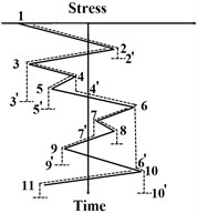
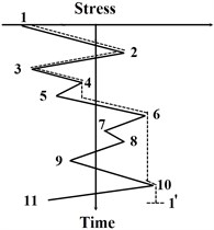
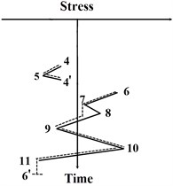
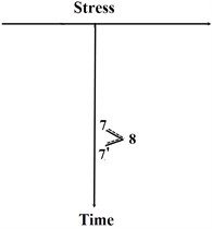
The modification in the MRFC method is to count cycles using a three-peak-trough counting algorithm, which can effectively avoid half cycles in the final statistical results. The detailed improvements in the computational process are provided below and sketched in Fig. 3,
a) The stress-time history is rotated clock-wise with 90° similar to the classical RFC method, such that the time axis is in vertical direction with the origin on the top and the positive direction points downward. Then, distinguished from the classical RFC method, the stress-time history in the MRFC method is regarded as multi-layer pagoda roofs. Since a raindrop begins to flow right from a trough or left from a peak onto subsequent roofs, the raindrop flow in the opposite direction when it is not blocked by a roof, e.g. path 1-2-3-4-6-10-1’ in Fig. 3(a). Thus, it can be called as a rain-flow cycle 1-6-1’. Then the maximum peak and trough values in the rain-flow path are recorded to calculate the stress range and mean stress.
b) The earlier rain-flow paths (e.g. path 1-2-3-4-6-10-1’) are deleted from the initial stress-time history and this operation is implemented in MATLAB (MathWorks, USA). The rest pagoda roofs are counted by the above-mentioned method, e.g. path 6-7-9-10-11-6’ that is also called as 6-10-6’.
Comparing to the counting process in the RFC method, the counting efficiency of the MRFC method is obviously improved while counting the same stress-time history. The efficiency and accuracy of the MRFC method will be validated in the following numerical cases in Section 5.
Fig. 3The counting process of the MRFC method
a) The first rain-flow path
b) The second rain-flow path
c) The third rain-flow path
2.3. Procedures for the whole fatigue damage analysis
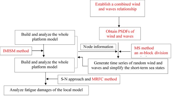
In the present study, a semi-submersible platform bears the combined actions of wind and waves. The complete computational procedures of fatigue damage analysis in time domain are summarized as follows and sketched in Fig. 4. In Fig. 4, all the improvements in the present work are marked with red fonts.
Step 1: build the whole model of the semi-submersible platform and the local model of key parts of the semi-submersible platform. The model information and the modeling method (e.g. the IMISM method) related to fatigue damage analyses are presented in Section 3. Meanwhile, export the finite-element grid node information (including node number and coordinates) as a txt file.
Step 2: generate time series of random wind and wave loads. A joint application of a combined wind and waves relationship and a proposed MS method is used to simulate the time series of random wind and waves of the finite-element grid nodes. Details of this step can be seen in Section 4. Then, the generated wind velocity-time histories and wave height-time histories can be converted, respectively, to time series of wind and wave loads of the corresponding nodes based on the current standards [23, 24] and the previous work [13, 32, 33]. An m-block division method in Section 4 is utilized to simply the short-term sea states for improving numerical efficiency.
Step 3: apply the time series of wind and wave loads on the corresponding finite-element grid nodes of the offshore structures by the Newmark- method with ANSYS Parametric Design Language (APDL, ANSYS, Inc., USA) [14]. Calculate the structural dynamic equations and export the structural dynamic responses (e.g. structural stresses) of the whole model and local model of the semi-submersible platform, which is also presented in Section 3.2 in detail.
Step 4: analyze the fatigue cumulative damage of the local components in each sea state based on the above-mentioned methods in this section and obtain the fatigue damage statistics of the local components.
Fig. 4The flow-chart for the whole fatigue damage analysis
3. The offshore platform model
Firstly, the detailed model information of a semi-submersible platform is presented in the first subsection. Then, the improved multiple interpolation sub-model (IMISM) method is proposed based on the sub-model method to analyze the structural dynamic responses of local model accurately, which is provided in the next subsection.
3.1. Model information
The whole model of a semi-submersible platform in the present study is a 6th generation deep-water drilling platform, and its main dimensions are recorded in Table 1 [13]. This whole model, as shown in Fig. 4, has five major components, from top to bottom, including a derrick, a deck, columns, horizontal braces and caissons. Structural modeling is realized by APDL similar to Cui et al. [7]’s modeling method. The beam, shell and volume elements are applied to generate the finite element model. The element size ranges from 0.25 m to 2 m.
Table 1The main dimensions of the semi-submersible platform
Members | Dimensions (length×width×height) / m |
Lower derrick | 17×17×42 |
Upper derrick | 17×17×22 |
Deck | 74.42×74.42×8.6 |
Column | 17.39×17.39×21.46 |
On the basis of the previous studies [6, 7], the fatigue damage evaluation relying only on the whole model in relatively coarse scale is not accurate enough. In order to guarantee the complexity and accuracy of the fatigue damage evaluation as well as to keep the total computational cost in check, the refined local model is built to analyze the fatigue damages of key parts in the semi-submersible platform [34]. According to the previous studies and practical experience [6, 7], the key parts are often prone to fatigue failure at the connections among the bars of the derrick, between the derrick and the columns, between the horizontal braces and the columns, between the caissons and the columns, especially at the connections between the horizontal brace and column, one of which is marked with a red circle in Fig. 5. Four connections are defined in sequence as: connection 1, 2, 3, 4. Therefore, the connection between the horizontal brace and the column is chosen in the present study and built as a refined local model, which is shown in Figs. 5(b) and 5(c). As depicted in Fig. 5(b), A, B, C and D are selected as the key nodes at the welding connection between the horizontal brace and the column to evaluate the fatigue damage of local components of a semi-submersible platform [21].
Fig. 5a) The whole model of a semi-submersible platform, b) the refined local model of one connection of the horizontal brace and column, c) four key nodes (A, B, C, D) at the welding connections of the refined local model
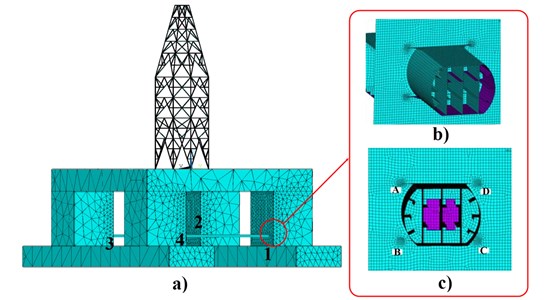
The boundary conditions applied on the local model are extracted from the wind and wave-induced structural responses of the whole model by the improved multiple interpolation sub-model (IMISM) method, which will be presented in detail in Section 3.2. This method is realized by the self-compiled secondary development programs in APDL in view of the basic idea of the sub-model method [34]. Thus, the modeling and mesh generation of the local model are the same as those of the whole model except that the element near four key nodes (i.e. A, B, C, D) should be refined as shown in Fig. 5(c).
3.2. The improved multiple interpolation sub-model (IMISM) method
The sub-model method, also called the cut-boundary interpolation method, focuses on precisely analyzing the local components of a whole finite element model as shown in Figs. 5(b) and (c), which has been proved to participate in analyzing structural fatigue damage [7, 34]. However, the cut-boundary in the sub-model method can only be volume and shell elements, which cannot satisfy the complex structural characteristics of a semi-submersible platform [34]. The IMISM method applied in the present work can solve this problem by APDL, whose applicability and accuracy have been validated in Cui [21]’s work.
The IMISM method mainly includes four parts, with the major considerations and improvements listed as follows:
a) Construct the whole model and analyze the dynamic response of the whole mode: Build the whole finite element model of a semi-submersible platform and calculate the wind- and wave-induced responses of the whole model [32-35].
b) Establish the local model: the local model is built using the proper elements in APDL. In the IMISM method, the stiffeners in the whole model are simulated with beam elements and the same stiffeners in the local model adopt shell elements. Extract the boundary conditions of the local model from the wind- and wave-induced responses of the whole model in step (a).
c) Perform the cut-boundary interpolations of the local model: Being different from the traditional cut-boundary interpolations in the sub-model method, the multiple interpolation in the IMISM method cuts two or more boundaries at the zones near the key nodes and carries out the cut-boundary interpolation by APDL to apply the boundary conditions on the local model.
d) Carry out the finite element analysis of the local model and output dynamic responses of A, B, C, D shown in Fig. 5(c) for the fatigue damage analysis.
4. Wind and waves loads
The section includes three improvements: In the first subsection, a combined wind and waves relationship is established in the present work and then the PSDFs of wind and waves are given in sequence. In the following subsection, a mixture simulation (MS) method is presented to simulate time series of the fluctuating wind and waves based on the above-given PSDFs of wind and waves. In the last subsection, an -block division method is proposed to compress the number of the whole short-term sea states, which can improve the efficiency of fatigue damage analyses in time domain.
4.1. A combined wind and waves relationship
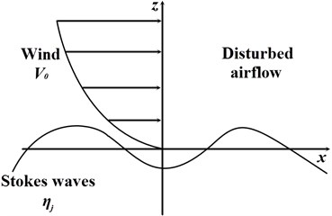
In this subsection, the combined relationship of wind and waves is explored based on the mechanism of wind generating Stokes waves [10-12]. Generally, ocean and sea environments are very complex and chaotic, mostly disturbed by atmospheric phenomenon. The disturbances on ocean surfaces are irregular water waves that are mostly generated by winds [36, 37]. When the wind has imparted its maximum energy to the waves, the sea is considered fully developed.
Based on the quasi-laminar model, the Stokes wave theory and the parallel flow instability theory [10, 11], the wind logarithm profile with the mean wind speed is disturbed by the surface elevation of Stokes waves in each order . The disturbing process is sketched in Fig. 6. The velocities and pressures in the disturbed airflow consist of the mean values and the disturbed values in each order [38]. Then, the governing equations of inviscid fluid without high order terms can be expressed as:
where and are the horizontal and vertical velocities, both and are the disturbed velocities, is the mean velocity, is the pressure, 1, …, , is the air density.
Fig. 6The sketch of the disturbance between wind and Stokes waves
Furthermore, the quasi-nonlinear energy transfer coefficient is introduced to explore the energy transfer relationship between wind and waves (ETR). The energy transfer in unit time and area is expressed as:
In which is the Stokes wave amplitude, is the only parameter related to energy transfer from wind to the Stokes waves, that is the above-mentioned quasi-nonlinear energy transfer coefficient. The numerical solutions of can be solved by implementing the fourth-order Runge-Kutta method [12, 41-42] in MATLAB.
Meanwhile, the mean total wave energy can be stated as:
where expectation is to calculate the expectation of the total transferred energy, is the gravitational acceleration, is the water density, and is the power spectral density function (PSDF) of the waves.
Since the fluctuating wind and waves are assumed as the stationary random Gaussian process, both of them can be described by the PSDF.
Based on Eq. (4), the total transferred energy can be written as:
where is a modified energy transfer coefficient only for 2 which is derived from , is the modified friction velocity of the airflow [40].
The IEC (International Electrotechnical Commission) Kaimal spectral equation is selected as the wind PSDF model in this subsection as follows:
where is the wind frequency, the standard deviation of velocity component, the integral scale parameter of velocity component, and the average wind velocity at the height of 10.0 m.
Therefore, the PSDF of wave can be derived from the ETR and the given wind PSDF. The derived equation is given as:
where is the wave frequency, is the modified frequency, ϑ is the adjusting coefficient of wave frequency, is the peak frequency, is the wave amplitude and is the peak adjusting coefficient.
Based on the above-provided PSDFs of wind and waves with a certain energy transferring relationship, the time series of fluctuating wind and waves can be simulated by the MS method which is presented in Section 4.2.
4.2. The mixture simulation (MS) method
In this subsection, the MS method is provided to generate time series of random wind and waves based on the above-proposed PSDFs of wind and waves in Eqs. (7, 8), respectively. This method in the present study combines the WAWS method with high numerical accuracy and the AR method with less time cost [14]. Thus, it becomes an efficient and accurate numerical simulation method for generating fluctuating wind and waves.
As is mentioned in Section 4.1, the random characteristics of wind and waves are described by the PSDFs of wind and waves. The main idea of the MS method is presented as follows: The energy distributions of the PSDFs of random wind or waves can be divided into energy dispersion and energy concentration parts by the wavelet method with adopting Hanning windows [43]. The equation can be expressed as:
where is the PSDF, is the frequency of wind or waves, and are respectively the Hanning windows of the energy concentration and dispersion, and are the corresponding energy concentration and dispersion parts of , respectively. According to Ma’s previous works [14, 44], simulate the time series of random wind or waves by the WAWS method, which can be considered as the time series . simulate the time series of random wind or waves by the AR method, which can be analogously called . The total time series of random wind or waves can be obtained by a linear superposition of and .
There is something worth mentioning here. In the MS method, the temporal and spatial correlations are adequately considered in the process of simulating the wind or wave-time histories of multiple spatial points in our MATLAB codes. The applicability, accuracy and efficiency of the MS method have been validated and the detailed derivation has been provided in our previous work [14].
4.3. An m-block division method
Fatigue damage analysis in time domain requires the structural stress response analysis of all sea states, which result in significant computational cost [21]. In this section, an -block division method combining some adjacent sea states in the wave-scatter diagram to generate fewer equivalent sea states is proposed. In the following numerical examples, this method demonstrates better numerical efficiency and sacrifices little accuracy. The basic idea of the -block division method is provided in Fig. 7.
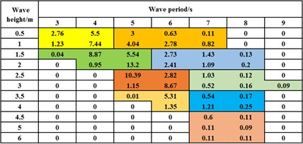
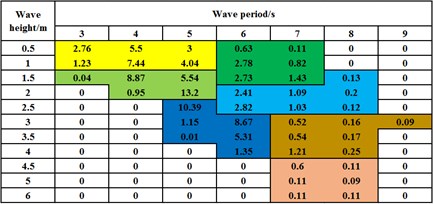
Fig. 7The grouping of all sea states by the m-block division method with m= 4 and m= 6 (one background color represents one analytical group): a) nine groups compressed by the m-block division method with m= 4, b) seven groups compressed by the m-block division method with m= 6
a)
b)
An -block division method combines adjacent sea states as one analytical group in the wave-scatter diagram, such as 4 or 6, whose operating results are shown in Figs. 7(a) and (b). Meanwhile, the different background colors represent different groups with the corresponding equivalent wave periods and heights. The first digit’s row and column are respectively wave period and height and other contents are the occurring probability of each sea state (the probability unit is %). Comparing to the traditional TDA method (i.e. 1), the -block division method with 4 and 6 decrease the required analytical group number from 43 to 9 and 7, respectively. It greatly minimizes the number of sea states and reduces the computational cost. The numerical efficiency is explored in the following numerical cases. For convenience, the -block division method with 4 and 6 are defined as 4-block division method and 6-block division method, and the traditional TDA method (i.e. 1) is also called as 1-division method.
Technically, 4-block division method or 6-block division method combines the adjacent four or six sea states together as one group. However, one group does not strictly consist of four or six sea states and can add or reduce one or two sea states when the occurring probabilities of one or two separate sea states are too small to be one separate group. For example, in the last row of Figs. 7(a) and (b), both the two sea states occur with a small probability of 0.11 % and cannot be a separate analytical group; Therefore, they are added to the last analytical group. Since the sea states in one group have different wave heights and periods, the corresponding equivalent wave height and period are calculated based on the following equations:
where is the equivalent wave period of each group, is the wave period of each sea state, is the probability of each sea state, is the equivalent spectral area of the wave PSDF of each group, is the spectral area of the wave PSDF of each sea state, where 1, …, and is the number of sea states in that group. According to the obtained and the corresponding wave heights of each sea state in this group, the equivalent wave height of each sea state in this group can be calculated by linear interpolation. The corresponding wind speed can be obtained by referring to the wave height and the combined relationship of wind and waves.
Finally, the analytical groups of all sea states compressed by 4-block division method and 6-block division method are utilized to calculate the structural stress responses for the structural fatigue damage analyses. The efficiency and accuracy of the -block division method with the proper comparing to 1-block division method are also investigated in the following section.
5. Results and discussion
In the section, the fatigue damages of the local components of a semi-submersible platform are analyzed and investigated by the ITDA method. The local components in the present study focus on the connections between the columns and horizontal braces. The above-mentioned improved method in the ITDA method are also discussed and validated by comparing to two traditional numerical methods (i.e. the time-domain analysis (TDA) method and the frequency-domain analysis (FDA) method) and the existing experimental data [23].
5.1. Validation test for the MRFC method
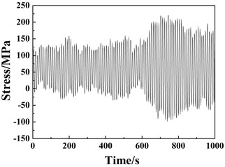
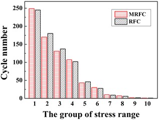
In this subsection, the reliability and applicability of the MRFC method are validated by comparing with the RFC method. A structural stress-time history is provided in Fig. 8(a) and the stress cycle statistics counted by the two methods is presented in Fig. 8(b).
Fig. 8a) A stress-time history extracted from the structural dynamic response of node A in Fig. 5(c), b) the corresponding stress cycle statistics by the MRFC and RFC methods
a)
b)
Based on the comparison between the counted results from the MRFC and RFC methods in Fig. 8, the maximum error is 6.67 % and the computational time using the MRFC method decreases by about 1/3 comparing to the RFC method (6.131s VS 9.192s).
Thus, to demonstrate the accuracy and efficiency of the MRFC method further, more time-structural stress histories of node A under different short-term sea states are extracted from dynamic structural response analyses in APDL and then counted by the RFC and MRFC method. Similar to Fig. 8(b), a series of stress ranges and corresponding cycle numbers are counted from one stress-time history curve by the RFC or MRFC method. Then, the cycle numbers corresponding to its stress range by the RFC and MRFC methods are a little different and compared to calculated its error by Eq. (12). Thus, the maximum errors can be compared and found from numerous sets of errors by Eq. (13), which are provided in Table 2:
where and are the cycle number of the th group of stress range in the th stress-time history curve by the MRFC method and RFC method, respectively. is the corresponding error of the th group of stress range in the th stress-time history curve:
where is the statistical maximum error, is an operator for seeking the maximum value.
The counting results are concluded in Table 2. Obviously, time cost in computation of the MFC method is steadily less than RFC method with the increasing number of the stress-time history curves. The data shows that the MRFC method reduces the time cost in computation by about 1/3 than the RFC method. However, the maximum errors are always ranging from 6 %, 7 %. Thus, it is concluded that the MRFC method is more efficient than the RFC method as well as sacrifices little accuracy. Therefore, the MRFC method is applicable in the present study.
Table 2Counting efficiency and accuracy of sometime-stress histories using RFC and MRFC methods
Number of time-stress histories | Time cost in computation / s | Maximum error / % | |
RFC | MRFC | ||
1 | 9.192 | 6.131 | 6.67 |
9 | 80.127 | 52.269 | 6.73 |
36 | 340.787 | 210.563 | 6.82 |
144 | 1312.535 | 861.763 | 7.01 |
5.2. Simulation and validation for wind and waves
The sea states for a combined wind and wave case have to be taken from a scatter block with three variables (i.e. wind speed, wave height and period), as shown in Fig. 9(a). The different colors in Fig. 9(a) represent the occurring probability of the wind and wave strength. The red color and blue color are the maximum and minimum probability, respectively. Fig. 9(a) consists of two parts: the wind speed and wave height relationship in Fig. 9(b) and a wave scatter with two variables (wave height and period) in Fig. 9(c). Based on the MS method and the given wind and waves model in Section 4, the wind speed and wave height relationship can be explored as shown in Fig. 9(b). The fitting curve of the numerical results are roughly in agreement with those provided by Kühn [45]’s work, especially wind speed less than 10 m/s. The errors are still within 12 % when wind speed exceeds 10 m/s. Fig. 9(c) is reproduced from the wave scatter diagram in [46, 47]. Fig. 9(c) can respectively be simplified by 4-block division method and 6-block division method and the simplifications are already provided in Figs. 7(a) and (b).
The equivalent wave height, wave period and probability in the analytical groups compressed by 4-block division method and 6-block division method are calculated as shown in Tables 3 and 4. Then, the corresponding wind speeds can be computed based on the wind speed and wave height relationship in Fig. 9(b). The equivalent results of wind speed are also listed in Tables 3 and 4. In any short-term sea state, the statistical characteristics of wind and waves can be fully defined by the PSDF.
Fig. 9a) The combined wind-wave scatter diagram with three variables, wind speed, wave height and periods, which consists of Figs. 8(b) and (c), b) the wind speed and wave height relationship diagram based on the combined relationship of wind and Stokes waves, c) the wave scatter diagram in [46, 47]
![a) The combined wind-wave scatter diagram with three variables, wind speed, wave height and periods, which consists of Figs. 8(b) and (c), b) the wind speed and wave height relationship diagram based on the combined relationship of wind and Stokes waves, c) the wave scatter diagram in [46, 47]](https://static-01.extrica.com/articles/18872/18872-img15.jpg)
a)
![a) The combined wind-wave scatter diagram with three variables, wind speed, wave height and periods, which consists of Figs. 8(b) and (c), b) the wind speed and wave height relationship diagram based on the combined relationship of wind and Stokes waves, c) the wave scatter diagram in [46, 47]](https://static-01.extrica.com/articles/18872/18872-img16.jpg)
b)
![a) The combined wind-wave scatter diagram with three variables, wind speed, wave height and periods, which consists of Figs. 8(b) and (c), b) the wind speed and wave height relationship diagram based on the combined relationship of wind and Stokes waves, c) the wave scatter diagram in [46, 47]](https://static-01.extrica.com/articles/18872/18872-img17.jpg)
c)
These parameters can be applied to simulate corresponding random wind and waves. Then, the stress responses of local components under the loading conditions are calculated by APDL [14].
Table 3The equivalent sea conditions compressed by the 4-block division method
Group number | Wave height / m | Wave period / s | Wind speed / (m/s) | Probability / % |
1 | 0.746 | 3.708 | 7.399 | 16.93 |
2 | 0.737 | 5.396 | 7.352 | 11.38 |
3 | 1.738 | 4.601 | 11.530 | 28.6 |
4 | 1.722 | 6.350 | 11.475 | 7.99 |
5 | 2.683 | 5.389 | 14.322 | 23.03 |
6 | 2.691 | 7.245 | 14.343 | 1.92 |
7 | 3.596 | 5.998 | 16.435 | 6.67 |
8 | 3.825 | 7.174 | 16.902 | 2.17 |
9 | 4.871 | 7.255 | 18.793 | 1.13 |
Table 4The equivalent sea conditions compressed by the 6-block division method
Group number | Wave height / m | Wave period / s | Wind speed / (m/s) | Probability / % |
1 | 0.757 | 4.013 | 7.455 | 23.97 |
2 | 1.191 | 6.248 | 9.465 | 8.5 |
3 | 1.736 | 4.601 | 11.523 | 28.6 |
4 | 2.234 | 6.337 | 13.092 | 7.8 |
5 | 2.946 | 5.525 | 14.978 | 26.88 |
6 | 3.608 | 7.227 | 16.460 | 2.94 |
7 | 4.871 | 7.255 | 18.793 | 1.13 |
5.3. Analyses and validation for the m-block division method
In this subsection, the ITDA method should determine the proper value of in the -block division method in comprehensive consideration of calculating efficiency and accuracy. The S-N curves in seawater with cathodic protection from “Recommended practice for fatigue strength analysis of offshore steel structure” [20] are used. The two-segmented S-N curve is given in Fig. 10.
Fig. 10The two-segmented S-N curve for the following fatigue damage analysis [6]
![The two-segmented S-N curve for the following fatigue damage analysis [6]](https://static-01.extrica.com/articles/18872/18872-img18.jpg)
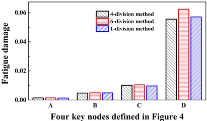
Using 1-block division, 4-block division and 6-block division methods, the short-term fatigue damage results under the incoming wind and wave angle 0° are compared to determine the proper value of . Fig. 11 depicts the comparisons of the numerical accuracy from the three methods. It is obviously shown that comparing to the 1-block division method, all the errors of the 4-block division method are less than those of the 6-block division method. The maximum error of the 4-block division method is 4.69 % and the other three errors range from 2 %-4 %. However, the maximum error of the 6-block division method is 10.6 % and the other three errors range from 7 %-9 %. Compared with the 1-block division method, the efficiencies of 4-block division and 6-block division methods are raised by more than 4 time and 5 times. Since it is only the numerical results under one wind and wave incoming angle, the total fatigue damage using the 6-block division method may have larger errors, the 4-block division method is the proper -block division method to be applied in the ITDA method.
Fig. 11The fatigue damage results of four key nodes defined in Fig. 4 under the incoming wind and waves angle 0°
5.4. Fatigue damage analyses
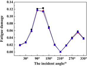
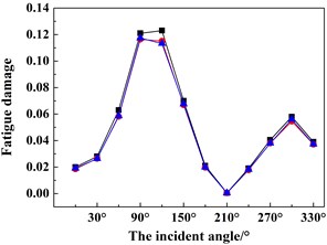
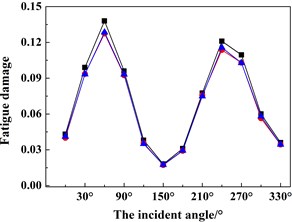
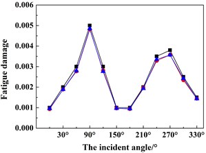
Based on the above-mentioned findings and discussions, Figs. 12(a)-(d) shows the fatigue damage results of the four key nodes (i.e. A, B, C, D) under 12 wind and wave incoming directions (i.e. 0°-330° with an interval of 30°). In order to validate the numerical accuracy of the ITDA method, the numerical results in Fig. 12 are simulated by the ITDA, TDA and FDA method. Meanwhile, the black lines with the black squares represent the fatigue damages results of the ITDA method; the red lines with the red spots are those of the TDA method; lastly, the blue lines with the blue triangles are those of the FDA method.
Seen from Fig. 12 firstly, the results of the ITDA are visually a little bit different from those of the TDA method and FDA method. The statistics data depicts that compared with the TDA and FDA method, the maximum errors are controlled within 7 % and 6.5 %. According to our computing and data process time, the total time cost of the ITDA method reduces to nearly 27.3 % of the TDA method and 68.7 % of the FDA method. It is concluded that the improved methods in the present study can efficiently save computing time with relatively similar results.
Observing Fig. 12 further, the changing trends of the fatigue damages are approximately similar with the change of wind and wave incident angles. The fatigue damages increase from 0° to 90° and then decease from 90° to 180°; The change from 180° to 360° is the same. In the up wind-wave state (i.e. 0° and 180°), the fatigue damages of all four key nodes are relatively less than those in the beam wind-wave state or in the oblique wind-wave state, especially in the beam wind-wave state. Therefore, for structural safety, the platform should keep in the up wind-wave state. Meanwhile, since all the fatigue damages are less than 1, this connection is safe and reliable.
Fig. 12The fatigue damage results under different incoming wind and waves angles of the four key nodes defined in Fig. 4 using the ITDA, TDA and FDA methods: a) the fatigue damage of node A, b) the fatigue damage of node B, c) the fatigue damage of node C, d) the fatigue damage of node D
a)
b)
c)
d)

According to the occurring probability of wind and wave incoming directions [46], the total fatigue damage of all four key nodes at connection 1 are calculated by the linear weighted method. There are four connections between the horizontal braces and columns in the present whole model, and then the fatigue damages of the four key nodes in the other three connections are calculated similarly. These fatigue damage results are presented in Table 5. All the fatigue damages are less than 1, which demonstrates the redundant safety of the structural members.
Lastly, in Fig. 13, the comparisons of the estimated fatigue life are presented to further verify the numerical accuracy and applicability. The estimated results come from the ITDA method, TDA method, FDA method and experimental evaluation [23] from left to right. It is found that the results of the ITDA and TDA methods are relative closer to the experimental evaluation. The design life in the experimental evaluation is defined as 30 years. Comparing to the experimental evaluation, the errors of the ITDA, TDA and FDA methods are 10.8 %, 11.5 % and 17.9 %, respectively. It is demonstrated that the ITDA method is applicable to analyze the fatigue damage of a semi-submersible platform.
Table 5The long-term fatigue damage results of all the connections between the columns and the horizontal braces
Connection number | Key nodes | Fatigue damage | Connection number | Key nodes | Fatigue damage |
1 | A | 0.014 | 3 | A | 0.044 |
B | 0.049 | B | 0.335 | ||
C | 0.097 | C | 0.137 | ||
D | 0.571 | D | 0.180 | ||
2 | A | 0.008 | 4 | A | 0.109 |
B | 0.025 | B | 0.146 | ||
C | 0.099 | C | 0.213 | ||
D | 0.046 | D | 0.080 |
Fig. 13The estimated fatigue life using four methods: a) the ITDA method, b) the TDA method, c) the FDA method, d) the experimental evaluation [23]
![The estimated fatigue life using four methods: a) the ITDA method, b) the TDA method, c) the FDA method, d) the experimental evaluation [23]](https://static-01.extrica.com/articles/18872/18872-img25.jpg)
6. Conclusions
The present study deals with the fatigue damage assessment of local components of a semi-submersible offshore platform subject to the combined wind and wave loads by a proposed improved time domain analysis (ITDA) method. The improvements of the ITDA method include combined wind and waves relationship, the mixture simulation (MS) method, the -block division method and the modified rain-flow counting (MRFC) method used in the loading conditions and the improved multiple interpolation sub-model (IMISM) method used in the modeling process. The explorations and computed results lead to the following conclusions:
1) An MRFC method is provided to count the stress-time history. A series of comparisons between the RFC and MRFC methods shows that the maximum error ranges from 6 % to 7 % with the increasing number of the stress-time history curves, however the MRFC method reduces the time cost in computation by about 1/3 than the RFC method. Therefore, the counting process of the MRFC method is more efficient with less accuracy lost comparing to the RFC method.
2) A combined relationship between wind and the Stokes waves is investigated and the PSDF of wind and waves are obtained. Using the MS method, the time series of wind or waves is generated, and the relationship of wind speed and wave height obtained in the present study is roughly in agreement with the previous published work [45], especially wind speed less than 10 m/s. The errors are still within 12 % when wind speed exceeds 10 m/s.
3) An -block division method is proposed to compress the number of the short-term sea states as fewer analytical groups. Compared with the 1-block division method, the 4-block division method can control the maximum error within 5 % and raise the efficiency by more than 4 times, which is a proper way to be applied in fatigue damage analyses.
4) Improving the sub-model method, an IMISM method can be used to analyze the structural stress responses of local components of the platform. The present study takes the connections between the horizontal brace and column as an example. Based on the S-N curve approach and cumulative fatigue damage rule, the fatigue damages of four connections between the horizontal braces and columns are calculated. Compared with the existing experimental data, the error of the estimated structural life by the ITDA method is less than that by the TDA method, 10.8 % versus 11.5 %. Under the combined actions of wind and waves, the fatigue damages of all key nodes are less than 1 and this platform has the redundant safety. The changing trends of the fatigue damages of all the key nodes are consistent: the fatigue damages increase from 0° to 90° and then decease from 90° to 180°; The change from 180° to 360° is the same. It is obviously found that their fatigue damages are the least under 0° and 180° (i.e. up wind-wave state). Therefore, it is recommended to adjust the platform in the up wind-wave state to slow down the fatigue damage accumulations.
References
-
Smith C.B. Extreme Waves. Joseph Henry Press, Washington, 2006.
-
Yao J. T. P., Kozin F., Wen Y. K., Yang J. N., Schuëller G. I., Ditlevsen O. Stochastic fatigue, fracture and damage analysis. Structural Safety, Vol. 3, Issue 3, 1986, p. 231-267.
-
Liuy M., Mahadevan S. Stochastic fatigue damage modeling under variable amplitude loading. International Journal of Fatigue, Vol. 29, Issue 6, 2007, p. 1149-1161.
-
Schijve J. Fatigue of structures and materials in the 20th century and the state of the art. Materials Science, Vol. 25, Issue 3, 2003, p. 679-702.
-
Hirdaris S. E., Bai W., Dessi D., Ergin A., Gu X., Hermundstad O. A., Huijsmans R., Iijima K., Nielsen U. D., Parunov J., Fonseca N., Papanikolaou A., Argyriadis K., Incecik A. Loads for use in the design of ships and offshore structures. Ocean Engineering, Vol. 78, 2014, p. 131-174.
-
Zha X. P. Theory and Method of Wind-Induced Fatigue Safety Prewarning for High-Rise Structure. Ph.D. Thesis, Wuhan University of Technology, 2008.
-
Cui L., Xu J. N., He Y., Jin W. L. Fatigue analysis on key components of semi-submersible platform. Proceedings of the 29th International Conference on Ocean, Offshore and Arctic Engineering, Shanghai, China, 2010.
-
Capanoglu C. Handbook of Offshore Engineering: Chapter 2 Novel and Marginal Field Offshore Structures. Plainfield, Illinois, 2005.
-
Kvittem M. I., Moan T. Time domain analysis procedures for fatigue assessment of a semi-submersible wind turbine. Marine Structures, Vol. 40, 2015, p. 38-59.
-
Miles J. W. On the generation of surface waves by shear flows. Journal of Fluid Mechanics, Vol. 2, 1957, p. 185-204.
-
Hristov T. S., Miller S. D., Friehe C. A. Dynamical coupling of wind and ocean waves through wave-induced air flow. Nature, Vol. 422, Issue 6927, 2003, p. 55-58.
-
Xu Y. Z., Li J. Stokes model for wind-wave interaction. Advances in Water Science, Vol. 2, 2009, p. 281-286, (in Chinese).
-
Ma J., Zhou D., Han Z. L. Wind and waves induced dynamic effects of a semi-submersible platform. The 27th International Offshore and Polar Engineering Conference, San Francisco, USA, 2017.
-
Ma J., Zhou D., Han Z. L., Zhang K., Nguyen J., Lu J. B., Bao Y. Numerical simulation of fluctuating wind effects on an offshore deck structure. Shock and Vibration, 2017, p. 3210271.
-
Chen J. L., Yang R. C., Ma R. L. Wind field simulation of large horizontal-axis wind turbine system under different operating conditions. Structural Design of Tall and Special Buildings, Vol. 24, 2015, p. 973-988.
-
Zang C. C., Christian J. M., Yuan J. K., Sment J., Moya A. C., Hob C. K., Wang Z. F. Numerical simulation of wind loads and wind induced dynamic response of heliostats. Energy Procedia, Vol. 49, 2013, p. 1582-1591.
-
Hill D., Bell K. R. W., Mcmillian D., Infield D. A vector auto-regressive model for onshore and offshore wind synthesis incorporating meteorological model information. Advances in Science and Research, Vol. 11, 2014, p. 35-39.
-
Karadeniz H. Stochastic Analysis of Offshore Steel Structures. Springer, London, 2013.
-
Rivero Angeles F.-J., Vázquez Hernández A.-O., Martinez U. Vibration analysis for the determination of modal parameters of steel catenary risers based on response-only data. Engineering Structures, Vol. 59, 2014, p. 68-79.
-
Larsen C. E., Irvine T. A review of spectral methods for variable amplitude fatigue prediction and new results. Procedia Engineering, Vol. 101, 2015, p. 243-250.
-
Yeter B., Grabatov Y., Soares C. G. Fatigue damage assessement of fixed offshore wind turbine tripod support structures. Engineering Structures, Vol. 101, 2015, p. 518-528.
-
Belloli M., Melzi S., Negrini S., Squicciarini G. Numerical analysis of the dynamic response of a 5-conductor expanded bundle subjected to turbulent wind. IEEE Transactions on Power Delivery, Vol. 2, Issue 4, 2010, p. 3105-3112.
-
Cui L. Fatigue Analysis of Deepwater Semi-Submersible Platform and Fatigue Test on Key Joint. Ph.D. Thesis, Zhejiang University, 2013.
-
Fatigue Design of Offshore Steel Structures. Det Norske Veritas, Oslo, 2010.
-
Guide for the Fatigue Assessment of Offshore Structures. American Bureau of Shipping, Houston, 2003.
-
Miner M. A. Cumulative damage in fatigue. Journal of Applied Mechanics, Vol. 12, Issue 3, 1945, p. 159-164.
-
Matsuishi M., Endo T. Fatigue of metals subjected to varying stress. Proceedings of Kyushi Branch JSME, Fukuoka, Japan, 1968.
-
Olagnon M., Guede Z. Rainflow fatigue analysis for loads with multimodal power spectral densities. Marine Structures, Vol. 21, 2008, p. 160-176.
-
Wang K. P., Xue H. X., Tang W. Y., Guo J. T. Fatigue analysis of steel catenary riser at the touch-down point based on linear hysteretic riser-soil interaction model. Ocean Engineering, Vol. 68, 2013, p. 102-111.
-
Yeter B., Garbatov Y., Soares C. G. Assessment of the Retardation of In-Service Cracks in Offshore Welded Structures Subjected to Variable Amplitude Load. Soares, C.G., Renewable Energies Offshore, Taylor & Francis Group, London, 2015, p. 855-863.
-
Low Y. M. Uncertainty of the fatigue damage arising from a stochastic process with multiple frequency modes. Probabilistic Engineering Mechanics, Vol. 36, Issue 2, 2014, p. 8-18.
-
Chakrabarti S. Handbook of Offshore Engineering: Chapter 4 Loads and Responses. Plainfield, Illinois, 2005.
-
Zhang R. Y., Tang Y. G., Hu J., Ruan S. F., Chen C. H. Dynamic response in frequency and time domains of a floating foundation for offshore wind turbines. Ocean Engineering, Vol. 60, 2013, p. 115-123.
-
ANSYS Inc. Advanced Analysis Techniques Guide. Canonsburg, Pennsylvania, USA, 2009.
-
Diana G., Fiammenghi G., Belloli M., Rocchi D. Wind tunnel tests and numerical approach for long span bridges: The Messina bridge. Journal of Wind Engineering and Industrial Aerodynamics, Vol. 122, 2013, p. 38-49.
-
Young W. R., Wolfe C. L. Generation of surface waves by shear-flow instability. Engineering Structures, Vol. 739, 2014, p. 276-307.
-
Ma J., Zhou D., Li F. F. Dynamic response and fatigue analysis of semi-submersible offshore platform with upper high-rise towers under combined wind and wave loads. Proceedings of the 14th International Symposium on Structural Engineering, Beijing, China, 2016.
-
Lyons T. The pressure in a deep-water stokes wave of greatest height. Journal of Mathematical Fluid Mechanics, Vol. 18, Issue 2, 2016, p. 209-218.
-
Atkins H. L., Hassan H. A. A new stream function formulation for the steady Euler equations. AIAA Journal, Vol. 23, Issue 5, 1983, p. 701-706.
-
Buckley M. P., Veron F. Structure of the airflow above surface waves. Journal of Physical Oceanography, Vol. 46, Issue 28, 2016, p. 1377-1397.
-
Conte S. D., Miles J. W. On the integration of the Orr-Sommerfeld equation. Journal of the Society for Industrial and Applied Mathematics, Vol. 7, Issue 4, 1959, p. 361-369.
-
Jenkins A. D. A Quasi-linear eddy-viscosity model for the flux of energy and momentum to wind waves using conservation-law equations in a curvilinear coordinate system. Journal of Physical Oceanography, Vol. 22, Issue 8, 2010, p. 843-858.
-
Testa A., Gallo D., Langella R. On the processing of harmonics and interharmonics using hanning window in standard framework. IEEE Transactions on Power Delivery, Vol. 19, Issue 1, 2004, p. 28-34.
-
Ma J. The Research of Wind Field and Fluid-Structure-Interaction and Fine Identification for Space Structure. Ph.D. Thesis, Shanghai Jiao Tong University, 2008.
-
Kühn M. Dynamics and Design Optimization of Offshore Energy Conversion Systems. Ph.D. Thesis, DUWIND Delft University Wind Energy Research Institute, 2003.
-
Zhou L., Wu L., Guo P. Simulation and study of wave in South China Sea using WAVEWATCH-III. Journal of Tropical Oceanography, Vol. 26, Issue 5, 2007, p. 1-8.
-
Zheng C. W., Zhuang H., Li X., Li X. Q. Wind energy and wave energy resources assessment in the East China Sea and South China Sea. Science China Technological Sciences, Vol. 55, Issue 1, 2012, p. 163-173.
About this article

This work was supported by the National Natural Science Foundation of China (Grant Nos. 51679139, 51490674 and 51278297); Research Program of Shanghai Leader Talent (Grant No. 20); Doctoral Disciplinary Special Research Project of Chinese Ministry of Education (Grant No. 20130073110096); and Natural Science Foundation of Shanghai (Grant No. 17ZR1415100).
