Abstract
This paper presents a novel variable stiffness isolator designed by magnetic springs in parallel with linear positive stiffness spring. Firstly, the two-degree-of-freedom vibration system model with variable stiffness magnetic isolator is established. The amplitude frequency characteristic equation of the system is derived based on the multi-harmonic method, and the corresponding curve of the relationship between the amplitude and frequency is given. The influence of the current on the curve is researched. Results showed that there are two pseudo-resonant peaks in the amplitude–frequency curve, and one is in the low frequency band, the other exists in higher frequency band. The first peak does not exhibit the frequency shift, but the second one bends to the natural frequency obviously. With the increasing of the current, the peaks decrease and the backbone curve changes greatly for the second resonant crest. The Lyapunov exponent curve around the resonant frequency is calculated. It is shown that there is chaotic parameter region for the system, and chaos can be controlled with the variable stiffness magnetic vibration isolator according to this research, which is beneficial to the design of nonlinear vibration isolation system.
1. Introduction
The design of high-static-low-dynamic stiffness isolator has always been the main target in practical engineering. For the vibration isolation system with high-static-low-dynamic stiffness, it can reduce the linear spectra well in the low frequency band. In order to obtain the high-static-low-dynamic stiffness isolator, the quasi-zero-stiffness (QZS) system including negative stiffness structure is required urgently. There are a number of ways to achieve negative stiffness, but the vast majority is passive. The typical structure is that two inclined springs are connected in parallel with a vertical spring [1-4]. Le [5] designed a quasi-zero-stiffness vibration isolation system by combining the two connecting-rods with the spring, and applied it to the vibration isolation of automobile seat. Results show that vibration suppression is effective of significantly. Carrella [6, 7] designed a high-static-low-dynamic stiffness isolator by using magnets and linear mechanical springs. Meng [8, 9] designed a new QZS isolator by connecting a disk spring with a linear spring, and studied the influence of system parameters on the transmissibility by using averaging method. Huang [10] proposed a method to design a QZS system by using a linear spring in parallel with an Euler beam as negative stiffness. Xu [11] proposed a new model of QZS isolator by combing two symmetrical magnetic negative stiffness springs with a vertical linear spring. Zheng [12] proposed a QZS isolator using a ring permanent magnet as negative stiffness structure. The above mentioned negative stiffness is realized by mechanical spring or permanent magnet, and the size cannot be adjusted. Therefore, a novel variable stiffness isolator designed by magnetic springs in parallel with linear positive stiffness spring is presented. The dynamic characteristics of a two-degree-of-freedom system consisting of variable stiffness magnetic isolator are analyzed and studied.
In the study of multi degree of freedom nonlinear vibration isolation system, the extraction of amplitude–frequency characteristic curve is an important part to analyze its dynamic characteristics. However, due to the existence of coupling between the degrees of freedom and the transfer of energy between nonlinear modes in high-dimensional nonlinear systems, the analysis and calculation are more difficult than the low-dimensional system. At present, it is rare to study the amplitude-frequency characteristics of the multi-degree-of-freedom nonlinear vibration isolation system and the control law of the system dynamics. In this paper, the dimensionless dynamical model of two-degree-of-freedom nonlinear vibration system consisting of a variable stiffness magnetic isolator is established, and the approximate expression of amplitude-frequency characteristic curve is deduced. The variation characteristics of the amplitude-frequency characteristic curve under different control current conditions are obtained, which is an important foundation for the control of nonlinear vibration.
2. Static analysis of the variable stiffness magnetic vibration isolator
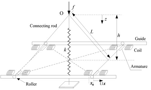
The configuration of the variable stiffness magnetic isolator considered in this paper is shown in Fig. 1. The magnetic spring is composed of electromagnet, armature and connecting rod. The magnetic springs act as a negative stiffness, connected with the mechanical spring at the position . Parameter is the vertical linear spring’s stiffness, is the length of the connecting rod, is the compression length of the vertical spring when the system reaches the static equilibrium position. The coordinate defines the displacement from the point .
Fig. 1Schematic of the variable stiffness magnetic isolator
Relationship between magnetic force and displacement is given by [13-15]:
where 0.03 m, 0.07 m, 0.008 m; is air permeability, ×10-7 H/m; is coil turns, 470; is area of magnet pole; is air gap between armature and electromagnet, 0.008 m; is armature displacement and is coil current.
Note that , the relational expression between the applied force and the displacement z is given by:
Introduce the non-dimensional parameters, , , , , Eq. (2) becomes:
Differentiating Eq. (3), the non-dimensional stiffness of the system can be obtained:
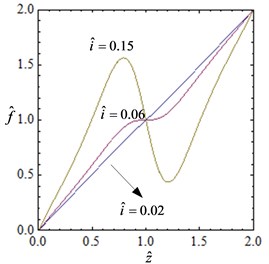
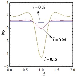
The current range of the coil is: A, then the non-dimensional current range is . Fig. 2 shows the curve of the non-dimensional force- displacement and stiffness- displacement for different currents. As shown in the Fig. 2, when the current is small, the system stiffness is approximately linear. With the increase of the current, the system exhibits obvious nonlinear characteristics.
3. Model of the two-degree-of-freedom system and amplitude-frequency equations
3.1. Model of the two-degree-of-freedom system
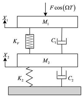
The model of the two-degree-of-freedom system is shown in Fig. 3. It includes the variable stiffness magnetic isolator between an upper mass and the middle mass ; a linear stiffness spring between the middle mass and the foundation. , are the vibration displacement; , are the system damping; is the excitation force amplitude; is the excitation frequency.
By using Taylor-series expansion, , expanding Eq. (3) at the static equilibrium position and substituting , an approximate expression of the non-dimensional force can be obtained:
where:
According to Newton’s law of motion, the system vibration equation is obtained:
Introducing the non-dimensional parameters, , , , , , , , .
The non-dimensional dynamic equation of the system can be expressed as:
Fig. 2The curve of the non-dimensional force-displacement and stiffness-displacement
a)
b)
Fig. 3Two-degree-freedom vibration system
3.2. Amplitude-frequency equations
Noting that , and yields:
The solution of the system is:
In order to facilitate analysis, set 1, inserting Eq. (10) into Eq. (9) and omitting higher order terms, yields:
The system response is projected on the basis functions consisting of sine and cosine functions, and yields:
Inserting Eq. (10), Eq. (11) and Eq. (12) into Eq. (9) and using the trigonometric function relation:
Set the coefficients of sine and cosine in Eq. (13b) to be zero:
Combing Eq. (14a) and Eq. (14b):
Inserting Eq. (15) into Eq. (13a) and eliminating the secular terms, the coefficients of sine and cosine can be obtained:
In order to satisfy the Eq. (13a), the constant term should be zero, and the higher order terms of are omitted:
0 can be get from Eq. (18). Introduce , , where is the response amplitude of the system. Eq. (16) and Eq. (17) become:
The amplitude-frequency relation expression can be obtained by the combination of Eq. (19) and Eq. (20) and application of 1:
4. Numerical simulations
4.1. Amplitude-frequency characteristics
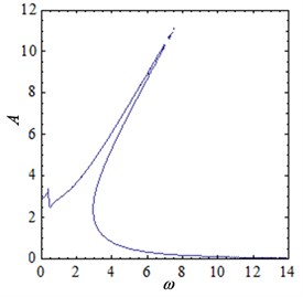
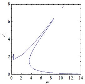
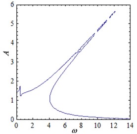
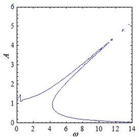
When parameters 0.2, 0.1, 0.2, 1.2, 1, 12, the current is 0.02, 0.04, 0.06 and 0.08, the amplitude-frequency curves of the two-degree-of-freedom isolation system are shown in Fig. 4. As can be seen from the Fig. 4, there are two pseudo-resonant peaks in the amplitude-frequency curve, and one is in the low frequency band, the other exists in higher frequency band. The first peak is the normal resonance peak, and the curve of the second resonance curves is obviously bent, that is, the resonance frequency shift occurs. It can be seen from the amplitude-frequency relationship Eq. (21) that the relationship between amplitude and frequency is not simple linear, so the phenomenon of multiple amplitudes at a frequency is presented. And the resonance curve is shifted at this time.
When the current increases from 0.02 to 0.04, the amplitude-frequency curve of the system is shown in Fig. 4(b). Compared with Fig. 4(a), the vibration peak is obviously reduced. The first resonance peak is reduced from 3.5 to 2.3, and the second resonance peak is reduced from 11.4 to 7.8. When the current increases to 0.06, the vibration peak is further reduced, as shown in Fig. 4(c). When the current increases to 0.08, the peak value of vibration remains downward. At the same time, it can be seen from Fig. 4 that with the increase of current, the bending degree of the curve becomes larger, which indicates that the nonlinear characteristics of the system are more and more obvious.
Fig. 4The amplitude-frequency curve of the system when current is varied
a) 0.02
b) 0.04
c) 0.06
d) 0.08
4.2. Chaotic vibration of the system
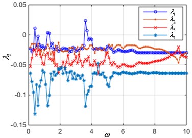
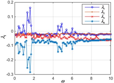
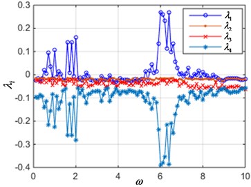
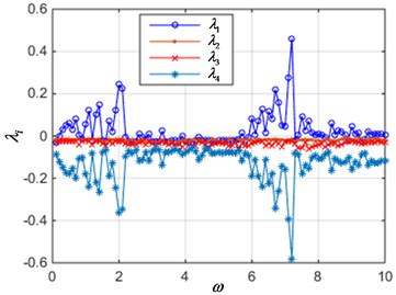
According to the previous analysis, the system shows obvious nonlinear characteristics. Especially, when the system is in the chaotic parameter region, it will produce chaotic vibration. Since the Lyapunov exponent is an important indicator to judge whether the system is in chaos. The Lyapunov exponent spectrum of the system can be calculated according to different parameters, thus providing the basis for chaotic identification.
When parameters 0.2, 0.1, 0.2, 1.2, 1, 12, the current is 0.02, 0.04, 0.06 and 0.08, the Lyapunov exponent curve of the system is shown in Fig. 5. It can be seen from the figures that when the current value is small, with the excitation frequency in the range of 0.1 to 10 changes, the interval of the positive maximum Lyapunov exponent curve is sparse, as shown in Fig. 5(a), which indicating that the system is in periodic motion parameters. As the current increases, the interval of the positive maximum Lyapunov exponent is gradually becoming denser. Especially in Fig. 5(d), the maximum Lyapunov exponent of the system is greater than zero in most parameter intervals, which indicates that the system moves from periodic motion to chaotic vibration. This is consistent with the analysis in Fig. 4.
According to the result of Fig. 5, when parameters 0.2, 0.1, 0.2, 1.2, 1, 12, the current is 0.02, 0.08 and the excitation frequency is 3.3, the phase diagram of the system is shown in Fig. 6. As can be seen from Fig. 6(a), (b), the system is in a periodic vibration state and the phase diagram is a limit cycle. From Fig. 6(c), (d), it can be seen that the system is in chaotic vibration state, and the phase diagram is a strange attractor. Therefore, the system under different control conditions will exhibit different nonlinear dynamic behaviors.
Fig. 5The Lyapunov exponent spectrum when current is varied
a) 0.02
b) 0.04
c) 0.06
d) 0.08
Fig. 6The phase diagram of the system
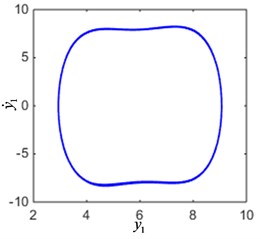
a) The limit cycle when 0.02
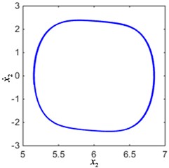
b) The limit cycle when 0.02
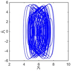
c) Chaotic response when 0.08
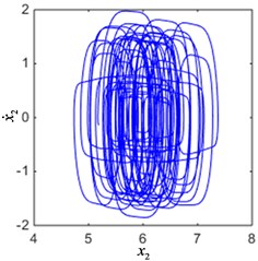
d) Chaotic response when 0.08
5. Conclusions
In this paper, a study of the two-degree-of-freedom nonlinear vibration system with a variable stiffness magnetic isolator has been presented. The mathematical model of the two-degree-of-freedom nonlinear vibration system is established. The approximate expression of the amplitude-frequency characteristic of the system is deduced, and the amplitude-frequency characteristic curve of the two-degree-of-freedom vibration system is obtained. The influence of the control current on the amplitude frequency characteristic curve is studied. It is observed that there are two pseudo-resonant peaks in the amplitude–frequency curve, and one is in the low frequency band, the other exists in higher frequency band. However, the region of the high frequency band has a tongue structure, which shows that there are nonlinear factors in the system. The resonance frequency shift phenomenon and the multi-amplitude characteristics at the same frequency are appeared. As the control current changes, the system's amplitude-frequency curve also changes. The specific rule is that when the control current increases, the resonance peaks of the system decrease, and the bending degree of the second resonance peak curve becomes larger. The curve of the Lyapunov exponent spectrum of the nonlinear system is calculated, and the chaotic parameter region of the system is obtained. The amplitude frequency characteristic curves of the system under the condition of chaotic parameters are analyzed. The results showed that the system can effectively be in the chaotic state under certain parameter conditions, and the linear spectrum can be effectively controlled.
References
-
Carrella A., Brennan M. J., Waters T. P. Static analysis of a passive vibration isolator with quasi-zero-stiffness characteristic. Journal of Sound and Vibration, Vol. 301, 2007, p. 678-689.
-
Kovacic I., Brennan M. J., Lineton B. Effect of a static force on the dynamic behavior of a harmonically excited quasi-zero stiffness system. Journal of Sound and Vibration, Vol. 325, 2009, p. 870-883.
-
Carrella A., Brennan M. J., Kovacic I. On the force transmissibility of a vibration isolator with quasi-zero-stiffness. Journal of Sound and Vibration, Vol. 322, 2009, p. 707-717.
-
Kovacic I., Brennan M. J., Waters T. P. W. A study of a nonlinear vibration isolator with a quasi-zero stiffness characteristic. Journal of Sound and Vibration, Vol. 315, 2008, p. 700-711.
-
Le T. D., Ahn K. K. A vibration isolator system in low frequency excitation region using negative stiffness structure for vehicle seat. Journal of Sound and Vibration, Vol. 330, Issue 26, 2011, p. 6311-6335.
-
Carrella A., Brennan M. J., Waters T. P. On the design of a high-static-low-dynamic stiffness isolator using linear mechanical springs and magnets. Journal of Sound and Vibration, Vol. 315, 2008, p. 712-720.
-
Carrella A., Brennan M. J., Waters T. P., et al. Force and displacement transmissibility of a nonlinear isolator with high-static-low-dynamic-stiffness. International Journal of Mechanical Sciences, Vol. 55, Issue 1, 2012, p. 22-29.
-
Meng L. S., Sun J. G., Wu W. J. Theoretical design and characteristics analysis of a quasi-zero stiffness isolator using a disk spring as negative stiffness element. Shock and Vibration, 2015, p. 1-19.
-
Niu F., Meng L. S., Wu W. J., et al. Design and analysis of a quasi-zero stiffness using a slotted conical disk spring as negative stiffness structure. Journal of Vibroengineering, Vol. 16, Issue 4, 2014, p. 1875-1891.
-
Huang Ch X., Liu X. T., Sun J. Y., et al. Vibration isolation characteristics of a nonlinear isolator using Euler buckled beam as negative stiffness corrector: a theoretical and experimental study. Journal of Sound and Vibration, Vol. 333, 2014, p. 1132-1148.
-
Xu D. L., Yu Q. P., Zhou J. X., et al. Theoretical and experimental analyses of a nonlinear magnetic vibration isolator with quasi-zero-stiffness characteristic. Journal of Sound and Vibration, Vol. 332, 2013, p. 3377-3389.
-
Zheng Sh Y., Zhang X. N., Luo Y. J., et al. Design and experiment of a high-static-low-dynamic stiffness isolator using a negative stiffness magnetic spring. Journal of Sound and Vibration, Vol. 360, 2016, p. 31-52.
-
Daley S., Johnson F. A. Active vibration control for marine applications. Control Engineering Practice, Vol. 12, 2004, p. 465-470.
-
Takeshi M., Masaya T., Daisuke K. Vibration isolation system combining zero-power magnetic suspension with springs. Control Engineering Practice, Vol. 15, 2007, p. 187-196.
-
Yeh T. J., Ying J. C. H., Wu W. C. Sliding control of magnetic bearing systems. Journal of Dynamic Systems, Measurement and Control, Vol. 123, 2001, p. 353-356.
About this article

This research is supported by the National Natural Science Foundation of China (51579242, 51509253, 51509255), and by Naval University of Engineering Foundation (425517K143). The authors wish to thank the reviewers for their careful, unbiased and constructive suggestions, which led to this revised manuscript.
