Abstract
The present paper provides mathematical model for the study of natural (free) vibration of non homogeneous tapered parallelogram plate on clamped boundary condition. Here non homogeneity (in material) of the plate’s means that the density and Poisson’s ratio varies circularly and exponentially respectively. For tapered, we assumed that thickness of the plate varies linearly in one direction. Bi parabolic temperature (parabolic in -direction and parabolic in -direction) variation on the plate is being viewed. Rayleigh Ritz method is used to solve the model (governing differential equation of motion).
1. Introduction
The study of vibration of tapered (non uniform) plates with non homogeneity in the material (non homogeneous plate) is the vast area of research due to its utility in various engineering applications like marine engineering, ocean engineering, optical instruments and mechanical engineering. Non homogeneous tapered plate plays significant role in engineering structures because of high tensile strength, durability and elastic behavior. All the engineering structure worked under great influence of temperature which causes non homogeneity. Therefore, with-out consideration of temperature the study of vibration means nothing. A significant work has been reported in these directions.
An excellent work on vibration of plates with various shapes has been described by Chakraverty [1]. Chen et al. [2] discussed the free vibration of cantilevered symmetrically laminated thick trapezoidal plates. Gupta and Mamta [3] studied non linear thickness variation of non homogeneous rectangle plate using spline technique. Free vibration has been discussed by Gupta and Sharma [4] on trapezoidal plate with thickness variation under temperature effect. Rotary inertial effect in isotropic plates (uniform and tapered thickness) has been carried out in two companion papers by Kalita et al. [5, 6]. The study of vibration of non uniform and non homogeneous rectangular plate with temperature effect has been studied by Khanna and Kaur [7-9] with exponential variation in non homogeneity. Leissa [10] provided vibration of plates (of different shapes) on different combination of boundary (clamped, simply supported and free) conditions in his excellent monograph. Leissa et. al. [11, 12] studied approximate analysis of the forced vibration response of plates and vibration of completely free triangular plates. Transverse vibration and instability of an eccentric rotating circular plate is studied by Ratko [13]. Sharma et al. [14-16] discussed natural vibration on orthotropic non homogeneous of rectangular plate, non homogeneous square plate (with circular variation in density) and non homogeneous trapezoidal plate with temperature effect.
The literature shows that the significant work has been done on vibration of non uniform (tapered) and non homogeneous plates with thermal gradient. Literature also emphasis on that, for non homogeneity either density or Poisson’s ratio varies linearly, parabolic and exponentially. But none of the researcher focused on other variation. This aspect provides good motivation to us to study the effect of circular variation in density as a new interesting aspect to frequency modes. Author also studies the effect of exponential variation in Poisson’s ratio as another parameter of non homogeneity (i.e., simultaneous variation in density and Poisson’s ratio) with the help of this model.
The model presented in this paper computes the vibrational frequency modes (first two modes) of non uniform and non homogeneous clamped parallelogram plate. This model also provides effect of other aspects such as effect of temperature and thickness to frequency modes.
2. Analysis
2.1. Description of model
A non uniform and non homogeneous parallelogram (thin) plate having skew angle is shown in Fig. 1.
The skew coordinates for the parallelogram plate are:
The boundaries of the plate in skew coordinates are:
For natural (free) vibration of plate, deflection (displacement) is assumed as [8]:
where and are known as maximum deflection (displacement) at time and time function respectively.
The differential equation of motion (kinetic energy and strain energy ) for natural frequency of non uniform parallelogram plate is given by [10]:
where , and are known as density, Poisson’s ratio and thickness of the plate. Here is known flexural rigidity; is Young’s modulus.
2.2. Assumptions for the model
Due to the wide range and general scope of vibrations, we require little limitations in the form of assumptions in this study.
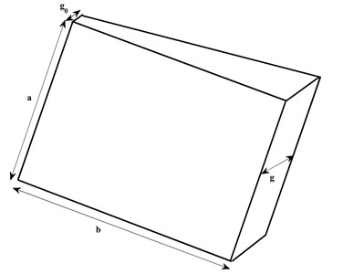
1) The thickness of the plate is assumed to be linear in -direction as shown in Fig. 2 as:
where , is known as tapering parameter. Thickness of plate become constant i.e., at .
Fig. 1Parallelogram plate with skew angle θ
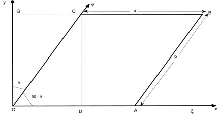
Fig. 2Tapered parallelogram plate
2) For non homogeneity in plate’s material, we taken into consideration that the density and Poisson’s ratio of the plate varies circularly and exponentially in -direction:
where , , are known as non homogeneity constant corresponding to density and Poisson’s ratio respectively.
3) The variation of temperature on the plate is considered as bi parabolic i.e., parabolic in and parabolic in direction:
where and denotes the temperature excess above the reference temperature on the plate at any point and at the origin respectively. The temperature dependence modulus of elasticity for engineering structures is given by:
where is the Young’s modulus at mentioned temperature (i.e., ) and is called slope of variation.
Using Eq. (9), Eq. (10) becomes:
where , is called temperature gradient, which is the product of temperature at origin and slope of variation i.e., .
Using Eqs. (6), (8) and (11), flexural rigidity of the plate becomes:
Also, using Eqs. (6), (7), (8) and (12), Eqs. (4) and (5) becomes:
In this model, we are computing frequency on clamped (along all the four edges) condition (i.e., on C-C-C-C), therefore the boundary conditions are:
Therefore, two term deflection (i.e., maximum displacement) which satisfy the Eq. (15) could be represented by:
where and are arbitrary constants.
3. Solution of model for frequency equation
To solve the model (obtain equation of frequency and vibrational frequency), we use Rayleigh Ritz technique (i.e., maximum strain energy must equal to maximum kinetic energy ). Therefore, we have:
Using Eqs. (13), (14) (15) and (16), Eq. (17) becomes:
where:
Here is known as frequency parameter. Eq. (18) consists of two unknown constants and (because of substitution of deflection function ). These two unknowns could be calculated as follows:
After simplifying Eq. (19), we get system of homogeneous equation as:
To obtain non-zero solution (frequency equation), the determinant of coefficient matrix (symmetric matrix) of Eq. (20) must zero i.e.:
Eq. (21) is quadratic equation from which we get two modes as (first mode) and (second mode).
4. Results and discussions
To examine the behavior of modes and effect of plate’s parameters (non homogeneity , , temperature gradient and tapering parameter ), numerical computation for frequency is carried out for different combination of plate’s parameters. The value of is taken 0.345. All the numerical computation is done with the help of MAPLE (high level software). All the findings are presented with the help of tables and graphs.
Table 1 provides the frequency modes (first two modes) corresponding to non homogeneity constant (corresponding to Poisson’s ratio and keeping density parameter off) with fixed value of skew angle 30° and aspect ratio 1.5 for three different values of taper constant and temperature gradient. i.e., 0, 0.4, 0.8. From Table 1, we conclude that frequency for both modes increases, when the non homogeneity corresponding to Poisson’s ratio increases from 0 to 1 for all the three values of taper constant and temperature gradient ( 0, 0.4, 0.8). Also, when the combined value of taper constant and temperature gradient increases from 0 to 0.8, frequency modes increases. The rate of increment in case of non homogeneity is much smaller (due to exponential variation) than the rate of increment in case of combined value of taper constant and temperature gradient .
Table 1Non homogeneity constant corresponding to Poisson’s ratio (m2) vs. frequency parameter (λ) for m1= 0, θ= 30° and a/b= 1.5
0.0 | 0.4 | 0.8 | ||||
0.0 | 78.77 | 313.60 | 86.28 | 343.38 | 90.68 | 360.69 |
0.2 | 79.94 | 318.24 | 87.63 | 348.77 | 92.14 | 366.65 |
0.4 | 81.45 | 324.25 | 89.40 | 355.87 | 94.08 | 374.58 |
0.6 | 83.44 | 332.14 | 91.76 | 365.31 | 96.71 | 385.31 |
0.8 | 86.07 | 342.59 | 94.94 | 378.05 | 100.28 | 399.98 |
1.0 | 89.60 | 356.61 | 99.24 | 395.40 | 105.16 | 420.26 |
Table 2 provides the different set of data (frequency modes) corresponding to non homogeneity constant (variable value of Poisson’s ratio and fixed value of density parameter 0.6) with fixed value of skew angle 30° and aspect ratio 1.5 for three different values of taper constant and temperature gradient. i.e., 0, 0.4, 0.8. From Table 2, one can easily see that the frequency behaviour (increases corresponding to non homogeneity and corresponding to combined value of thermal gradient and taper constant) is same as in Table 1. But due to implementation of another non homogeneity parameter (circular variation in density parameter) the frequency modes are less when compared to Table 1.
Table 2Non homogeneity constant corresponding to Poisson’s ratio (m2) vs. frequency parameter (λ) for m1= 0.6, θ= 30° and a/b= 1.5
0.0 | 0.4 | 0.8 | ||||
0.0 | 75.41 | 298.54 | 82.51 | 325.99 | 86.65 | 341.73 |
0.2 | 76.53 | 302.96 | 83.79 | 331.11 | 88.04 | 347.37 |
0.4 | 77.98 | 308.68 | 85.49 | 337.85 | 89.90 | 354.88 |
0.6 | 79.88 | 316.18 | 87.75 | 346.81 | 92.41 | 365.04 |
0.8 | 82.40 | 326.14 | 90.79 | 358.90 | 95.83 | 378.93 |
1.0 | 85.78 | 339.48 | 94.91 | 375.36 | 100.50 | 398.13 |
Table 3 gives frequency modes corresponding to non homogeneity constant (corresponding to density parameter and keeping Poisson’s ratio off) with fixed value of skew angle 30° and aspect ratio 1.5 for three different values of taper constant and temperature gradient. i.e., 0, 0.4, 0.8. From Table 3, we enlighten the fact that frequency for both decreases, when the non homogeneity corresponding to density parameter increases from 0 to 1. Here the frequency behave totally opposite (decreases corresponding to ) to Table 1 (increases corresponding to ). On the other hand frequency increases when the combined value of taper constant and temperature gradient increases from 0 to 0.8 as in Table 1. Here the rate of decrement is much smaller (due to circular variation) as compared to rate of increment in Table 1.
Table 4 provides the another set of data (frequency modes) corresponding to non homogeneity constant (variable value of density parameter and fixed value of Poisson’s ratio 0.6) with fixed value of skew angle 30° and aspect ratio 1.5 for three different values of taper constant and temperature gradient. i.e., 0, 0.4, 0.8. From Table 4, one can easily get that frequency behaves same as in Table 3 (in all respect). But due to the implementation of other non homogeneity constant (exponential variation in Poisson’s ratio) the frequency for both modes is higher when compared to Table 3. Here the rate of decrement is same as in Table 3 because of circular variation in density parameter.
Table 3Non homogeneity constant corresponding to density (m1) vs. frequency parameter (λ) for m2= 0, θ= 30° and a/b= 1.5
0.0 | 0.4 | 0.8 | ||||
0.0 | 78.77 | 313.60 | 86.28 | 343.38 | 90.68 | 360.69 |
0.2 | 77.60 | 308.33 | 84.97 | 337.27 | 89.28 | 354.02 |
0.4 | 76.48 | 303.32 | 83.71 | 331.49 | 87.94 | 347.71 |
0.6 | 75.41 | 298.54 | 82.51 | 325.99 | 86.65 | 341.73 |
0.8 | 74.38 | 293.99 | 81.35 | 320.77 | 85.42 | 336.05 |
1.0 | 73.40 | 289.64 | 80.25 | 315.79 | 84.25 | 330.65 |
Table 5 accommodates the frequency modes corresponding to thermal gradient with fixed value of non homogeneity constant (corresponding to Poisson’s ratio ), skew angle 30° and aspect ratio 1.5 for three different values of non homogeneity constant (correspondint to density) and tapering parameter i.e., 0.2, 0.4, 0.8. From Table 5, it is interesting to note that when the temperature gradient on the plate increases from 0 to 0.8, frequency modes decreases for the all the three values of non homogeneity constant and tapering paramenter . Also, when the combined values of non homogeneity corresponding to density and tapering parameter increases from 0.2 to 0.8, the frequency modes also increases.
Table 4Non homogeneity constant corresponding to density (m1) vs. frequency parameter (λ) for m2= 0.6, θ= 30° and a/b= 1.5
0.0 | 0.4 | 0.8 | ||||
0.0 | 83.44 | 332.14 | 91.76 | 365.31 | 96.71 | 385.31 |
0.2 | 82.20 | 326.55 | 90.36 | 358.82 | 95.21 | 378.17 |
0.4 | 81.01 | 321.24 | 89.03 | 352.66 | 93.78 | 371.43 |
0.6 | 79.88 | 316.18 | 87.75 | 346.81 | 92.41 | 365.04 |
0.8 | 78.79 | 311.36 | 86.52 | 341.25 | 91.10 | 358.97 |
1.0 | 77.75 | 306.75 | 85.35 | 335.95 | 89.85 | 353.20 |
Table 5Thermal gradient (α) vs. frequency parameter (λ) for m2= 0, θ= 30° and a/b= 1.5
0.2 | 0.4 | 0.8 | ||||
0.0 | 85.47 | 339.42 | 92.17 | 364.85 | 105.38 | 414.25 |
0.2 | 81.58 | 324.07 | 88.05 | 348.57 | 100.80 | 396.14 |
0.4 | 77.49 | 307.96 | 83.71 | 331.49 | 95.98 | 377.17 |
0.6 | 73.14 | 290.97 | 79.11 | 313.48 | 90.87 | 357.20 |
0.8 | 68.49 | 272.92 | 74.19 | 294.39 | 85.42 | 336.05 |
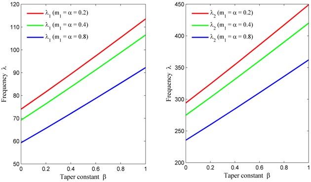
When we look at the Table 6, it tells how frequency modes behave for the fixed value of non homogeneity constant (Poisson’s ratio 0), skew angle 30°, aspect ratio 1.5 and variable value of non homogeneity constant (density parameter 0.2, 0.4, 0.8) and temperature gradient ( 0.2, 0.4, 0.8) corresponding to tapering parameter of the plate. From the Table 6, we enlighten the fact that when the tapering parameter of the plate increases from 0 to 1, modes of frequency increases (due to linear variation in thickness). On the other hand, when the combined value of density parameter and temperature increases from 0.2 to 0.8, modes of frequency decreases.
In order to get good understanding of results and discussions (variation of plate’s parameter), graphical representation of Tables 1-6 presented in the form of Figs. 3-9.
Table 6Taper constant (β) vs. frequency parameter (λ) for m2= 0, θ= 30° and a/b= 1.5
0.2 | 0.4 | 0.8 | ||||
0.0 | 74.00 | 294.18 | 69.19 | 274.76 | 59.30 | 235.40 |
0.2 | 81.58 | 324.07 | 76.36 | 302.80 | 65.62 | 259.84 |
0.4 | 89.37 | 354.65 | 83.71 | 331.49 | 72.11 | 284.85 |
0.6 | 97.31 | 385.75 | 91.20 | 360.66 | 78.72 | 310.28 |
0.8 | 105.37 | 417.25 | 98.81 | 390.22 | 85.42 | 336.05 |
1.0 | 113.52 | 449.07 | 106.50 | 420.08 | 92.20 | 362.08 |
Fig. 3Non homogeneity constant (m2) vs. frequency (λ) for fixed m1= 0, θ= 30° and a/b= 1.5
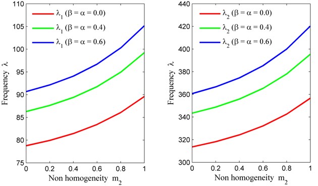
Fig. 4Non homogeneity constant (m2) vs. frequency (λ) for fixed m1= 0.6, θ= 30° and a/b= 1.5
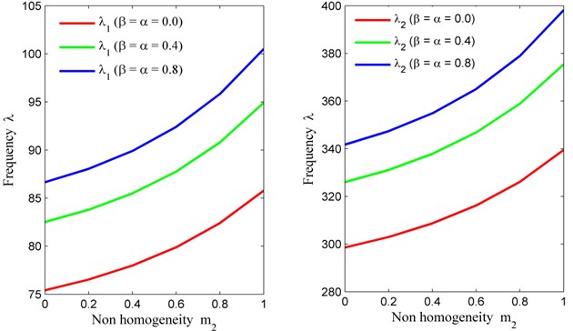
Fig. 5Non homogeneity constant (m1) vs. frequency (λ) for fixed m2= 0, θ= 30° and a/b= 1.5
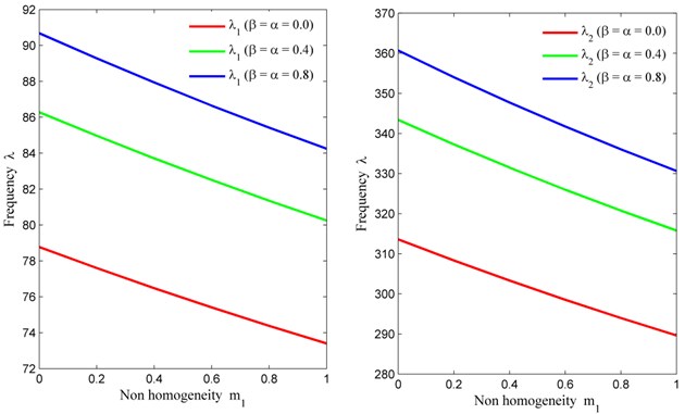
Fig. 6Non homogeneity constant (m1) vs. frequency (λ) for fixed m2= 0.6, θ= 30° and a/b= 1.5
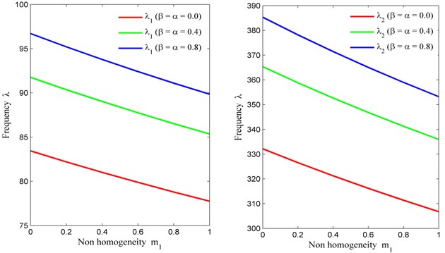
Fig. 7Thermal gradient (α) vs. frequency (λ) for fixed m2= 0, θ= 30° and a/b= 1.5
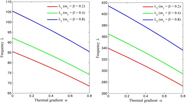
Fig. 8Taper constant (β) vs. frequency (λ) for fixed m2= 0, θ= 30° and a/b= 1.5
5. Conclusions
This model display the effect of plate’s parameter on vibration of non homogeneous tapered parallelogram plate (with the help of Tables 1-6 and Figs. 3-8). With the help of this model, author drags the attentions of the readers on two important aspects. Firstly, effect of simultaneous variation of Poisson’s ratio and density parameter (as non homogeneity effect) to vibrational frequency (in Table 2 and Table 4). The frequency is less in Table 2 (due to circular variation in density parameter) as compared to Table 1 (density parameter is off). The frequency is high in case of Table 4 (due to exponential variation in Poisson’s ratio) when compared to Table 3. Secondly, effect of circular variation in density to vibrational frequency (in Table 3). The frequency is decreasing corresponding to density parameter (in Table 3). But frequency is increasing corresponding to Poisson’s ratio (in Table 1). The rate of decrement/increment in frequency is less in Table 3 when compared to Table 1. The author also provides effects of temperature (in Table 5) and thickness (in Table 6) to vibrational frequency. This paper gives good appropriate numerical data of frequency modes which is helpful for researchers and scientists, making good optimal structural designs.
References
-
Chakraverty S. Vibration of Plates. CRC Press, Boca Raton, 2008.
-
Chen C. C., Kitipornchai S., Lim C. W., Liew K. M. Free vibration of cantilevered symmetrically laminated thick trapezoidal plates. International Journal of Mechanical Sciences, Vol. 41, 1999, p. 685-702.
-
Gupta A. K., Mamta Non-Linear thickness variation on the thermally induced vibration of a rectangular plate: a spline technique. International Journal of Acoustics and Vibration, Vol. 19, Issue 2, 2014, p. 131-136.
-
Gupta A. K., Sharma P. Vibration study of non-homogeneous trapezoidal plates of variable thickness under thermal gradient. Journal of Vibration and Control, Vol. 22, Issue 5, 2016, p. 1369-1379.
-
Kalita K., Shivakoti I., Ghadai R. K., Haldar S. Rotary inertial effect in isotropic plates part I: uniform thickness. Romanian Journal of Acoustics and Vibration, Vol. 13, Issue 2, 2016, p. 68-74.
-
Kalita K., Shivakoti I., Ghadai R. K., Haldar S. Rotary inertial effect in isotropic plates part II: taper thickness. Romanian Journal of Acoustics and Vibration, Vol. 13, Issue 2, 2016, p. 75-80.
-
Khanna A., Kaur N. Theoretical study on vibration of non-homogeneous tapered visco-elastic rectangular plate. Proceedings of the National Academy of Sciences, India Section A: Physical Sciences, Vol. 86, Issue 2, 2016, p. 259-266.
-
Khanna A., Kaur N. Effect of thermal gradient on vibration of non-uniform visco-elastic rectangular plate. Journal of The Institution of Engineers (India): Series C, Vol. 97, Issue 2, 2016, p. 141-148.
-
Khanna A., Kaur N. Effect of structural parameter on vibration of non homogeneous visco elastic rectangular plate. Journal of Vibration Engineering and Technology, Vol. 4, Issue 5, 2016, p. 459-456.
-
Leissa A. W. Vibration of Plates. NASA SP-160, 1969.
-
Leissa A. W., Chern T. Y. Approximate analysis of the forced vibration response of plates. Journal of Vibration and Acoustics, Vol. 114, Issue 1, 1992, p. 106-111.
-
Leissa A. W., Jaber N. A. Vibration of completely free triangular plates. International Journal of Mechanical Sciences, Vol. 34, Issue 8, 1992, p. 605-616.
-
Ratko M. Transverse vibration and instability of an eccentric rotating circular plate. Journal of Sound and Vibration, Vol. 280, 2005, p. 467-478.
-
Sharma A., Sharma A. K., Raghav A. K., Kumar V. Effect of vibration on orthotropic visco-elastic rectangular plate with two dimensional temperature and thickness variation. Indian Journal of Science and Technology, Vol. 9, Issue 2, 2016.
-
Sharma A., Sharma A. K., Raghav A. K., Kumar V. Vibrational study of square plate with thermal effect and circular variation in density. Romanian Journal of Acoustics and Vibration, Vol. 13, Issue 2, 2016, p. 146-152.
-
Sharma A. K., Sharma A., Raghav A. K., Kumar V. Analysis of free vibration of non-homogenous trapezoidal plate with 2D varying thickness and thermal effect. Journal of Measurements in Engineering, Vol. 4, Issue 4, 2016, p. 201-208.
About this article

