Abstract
The sub-grade of the railway track subjected to dynamic loading is governed by its dynamic material parameters, the basic dynamic material parameters are unit weight, Young’s modulus, Poisson’s ratio and the material damping. However, there is a need to identify the parameters of the sub-grade that has significant effect on the dynamic response of the railway track to achieve the specified technical requirements because the behavior of the sub-grade cannot be easily estimated or verified. Hence, this paper uses three-dimensional finite elements ABAQUS coupled with Artificial Non-Reflecting Boundary to investigate the effect of varying the unit weight, Young’s modulus, Poisson's ratio and the damping ratio of the sub-grade in the surface vibration induced at the embankment railway track in terms of Peak Vertical Velocity due to moving of the train loads. The input soil parameters used are soft clay, stiff clay, loose and dense uniform sand to demonstrate the parametric study. The predicated results show that both the Young’s modulus and damping ratio of the sub-grade have quite significant effect on the induced surface vibrations of railway track; while the influence of both unit weight and Poisson’s ratio are very small. Hence to fulfill the technical requirement of the railway track, special attention regarding to the Young’s modulus and the damping ratio of the sub-grade should be paid.
Highlights
- A numerical model using ABAQUS was established to analyze train induced vibrations.
- Non-reflecting boundary was defined at the far end.
- The variation in surface vibrations by varying four different set of sub-grade parameters were evaluated
- The computational model is verified with the previous published work.
1. Introduction
Railway is regarded as one of the most crucial means of transportation and is widely used in several applications. Meanwhile, the infrastructure that carries the trains need to be understood to carry the vibration induced from moving train loads so as to alleviate disturbances in the structures, surrounding, and the significant deterioration of the adjacent sub-grades [1]. The maintenance and renewal costs of a typical railway track substructures represent 50-60 % of the total costs over its entire service life [2]. The sub-grade is the weakest and most unstable part in railway line works. If the sub-grade does not have sufficient stability, it will be impossible to maintain proper track alignment, profile (surface) and cross level.
In the last a few decades, many published reports have included the results of dynamic motion of sub-grade due to train operation. For instance, the effect of variable subsoil conditions has been studied [2], railway embankments on layered ground is studied [3], the dynamic behavior of the rail track has been examined [4], numerical modeling of ground borne vibrations from high speed rail lines on embankments is presented [5], three-dimensional dynamic analyses of track-embankment-ground system subjected to high speed train loads is developed [6] and prediction model for low frequency vibration from high speed railways on soft ground is observed [7]. Thus, the proposed models have been examined that the railway track is more vulnerable to larger deformations concentrated in the soft soil and shows a greater stability in case of stiff soils, but the studies did not consider the influence of material parameters.
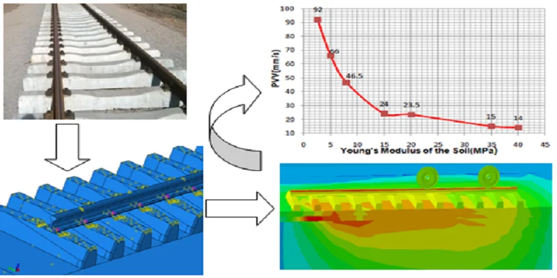
This paper mainly focused on the comparison of results obtained through numerical models of railway vibrations under different choice of sub-grade parameters. Therefore, we are looking for an attribute which can separate the influence of parameters from general soil types. Moreover, the goal is to identify the parameters that cause high vibration levels which have never been done in more detail manner so far, and evaluate the variation in the induced surface vibrations for different set of parameters. The analysis is performed using the commercial finite element package, ABAQUS after imported 3D solid elements from CATIA software.
Fig. 1a) Railway embankment in Ethiopia (Awash-Kombolcha-Haragebaya railway project), b) track with different components [8]
![a) Railway embankment in Ethiopia (Awash-Kombolcha-Haragebaya railway project), b) track with different components [8]](https://static-01.extrica.com/articles/18725/18725-img1.jpg)
a)
![a) Railway embankment in Ethiopia (Awash-Kombolcha-Haragebaya railway project), b) track with different components [8]](https://static-01.extrica.com/articles/18725/18725-img2.jpg)
b)
2. Modeling approach
2.1. Geometry of the model
In order to examine the sub-grade response due to the surface vibration a model involving all components of the track structure (rail, rail-pad, sleepers, substructures (ballast, sub-ballast and sub-grade), and vehicle parameters considering the axle spacing, axle load and diameter of the wheel are required. The track was modeled in a configuration similar to that found in newly built tracks in Ethiopia railway Projects. The rail used in this simulation was UIC-54 rail supported by concrete sleepers laid at 0.60 m centers. The sleepers were then supported by 0.15 m layer of ballast, 0.15 m layer of sub-ballast, finally 16 m sub-grade was considered. All the track components are modeled as three dimensional solid elements except the rail-pads. The rail pads were modeled as spring element which have vertical stiffness () and viscous damping ().
Due to excessive computational time to solve the 3-D dynamic problem through numerical models, only half of the track is modeled means symmetry with respect to the center line is assumed. The length of the track considered is limited to 12 sleepers based on Kumaran et al works [9] with two moving railcar wheels as indicated in [10]. Besides, the sleeper is considered as solid element. The slope of the embankment adopted in the model was 3.5.
Fig. 2Model of rail (UIC-54)
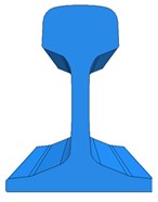
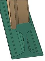
Fig. 3Model of half sleeper

2.2. Material model
The rail, sleeper, wheel, sub-ballast, ballast and the sub-grade are considered as linear elastic and damped material. The Young’s modulus () of the soil is varying with depth, the sub-grade soil was divided in 3 different layers; i.e. 2.5 m of the embankment, 2 m formation layer (Ground 1) and 11.5 m of base soil layers (Ground 2). In addition, the damping ratio for the soil varies from 1 % to 20 % [11]. Note that all the sub-grade parameters in Table 1 are the base set parameters. For further investigation they will be varied to determine their influence on the surface vibration levels. Generally, the sub-grade and subsoil layers used are shown below in Table 1.
Fig. 4Wheel-rail contact interface: a) model of wheel-rail contact, b) real-wheel-rail contact
a)

b)
Fig. 5Finite element model track overview (longitudinal view)
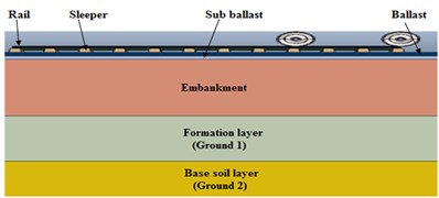
Table 1The material properties used for the subgrade and subsoil layers to implement the scenario
Component | Layer | (m) | (MPa) | [kg/m3] | (о) | (%) | |
Soft clay | Embankment | 2.5 | 2.5 | 1330 | 0.3 | 5 | 20 |
Ground 1 | 2.0 | 7.5 | 1330 | 0.3 | 5 | 20 | |
Ground 2 | 11.5 | 12.5 | 1330 | 0.3 | 5 | 20 | |
Stiff clay | Embankment | 2.5 | 15 | 1730 | 0.3 | 5 | 20 |
Ground 1 | 2.0 | 20 | 1730 | 0.3 | 5 | 20 | |
Ground 2 | 11.5 | 25 | 1730 | 0.3 | 5 | 20 | |
Loose sand | Embankment | 2.5 | 10 | 1470 | 0.3 | 24 | 20 |
Ground 1 | 2.0 | 15 | 1470 | 0.3 | 24 | 20 | |
Ground 2 | 11.5 | 20 | 1470 | 0.3 | 24 | 20 | |
Dense sand | Embankment | 2.5 | 50 | 1800 | 0.4 | 36 | 20 |
Ground 1 | 2 | 55 | 1800 | 0.4 | 36 | 20 | |
Ground 2 | 11.5 | 65 | 1800 | 0.4 | 36 | 20 |
2.3. Interface modeling
Surface-to-surface contact elements were model using master and slave surface interface elements. The basic Coulomb friction model with the penalty friction formulation was used to simulate the frictional force response at the contact interface. The model specifies the shear behavior in terms of normal and tangential [12]; i.e. , where. is the critical shear stress at contact surface, is the coefficient of friction and, is the contact pressure between the two surfaces. The maximum allowable frictional stress is related to contact pressure by coefficient of friction between contacting bodies [13].
Based on direct shear tests on various surface materials, Durgunoglu and Mitchell [14, 15], suggested using 0.5 for most penetration in practice, where Peak angle of effective internal friction and is the angle of interface friction. Besides, According to Susila and Hrychiw [16], coefficient of friction () between different components found to be a function of angle of internal friction; i.e. . The coefficient of friction between the substructure components of the track is assumed to be a function of angle of internal friction. The contact between wheel and rail, sleeper and rail, sleeper and granular soils is used as indicated in [17].
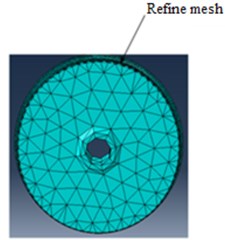
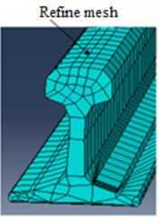
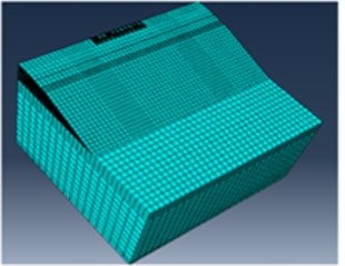
2.4. Element type and mesh size
The track components were modeled using linear four-node tetrahedron and Eight-node linear brick elements with 3D deformable solid. Refined elements were used on the railhead contact with wheel sets and perimeter of the wheel tread, since the vibration is predominantly induced by the interaction between the moving wheels and rails [18]. Four mesh sizes with the element size of 0.05 m, 0.15 m and 0.75 m and 1 m were considered.
Fig. 6Mesh detail: a) wheel, b) rail, c) isometric view of the whole model
a)
b)
c)
2.5. Loading procedure
The axle load and spacing used for simulations can be different in various literatures. Nevertheless, the Ethiopia Railways Corporation used two axle loads of 250 kN and 1.83 m axle spacing for design of rail seat load for the case of freight car. Accordingly, two moving wheel loads of 125 kN are applied, which are 1.83 m apart in order to model the passage of freight car on a conventional line. The wheel loads remain for 0.03 s in its starting position during loading. After 0.03 s the wave induced by the mass loading have disappeared, do not affect the results anymore and the load variation in the initial state was removed. Afterwards the wheel starts to move along the rail for 0.178 s. The computation must end later, in order to stabilize the vibrations in the surrounding media. Hence, the remaining load parameters 0.292 s were used to stabilize the vibrations. The maximum necessary displacement imposed by the boundary condition manager is 4.94 m, obtained for the speed of 120 km/h. In general, the following steps were used to apply the train loads and to study the dynamic response of sub-grade of the track system.
2.6. Boundary conditions
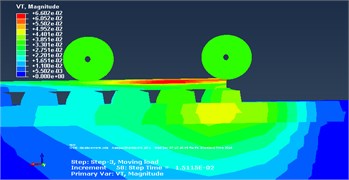
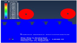
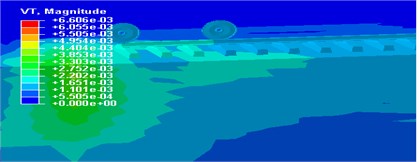
To minimize unrealistic reflections of the waves from the boundary, Artificial Non-Reflecting Boundary was defined at the far end of the model. For the implementation of Artificial Non-Reflecting boundary, a region in 8 m width is added to the end of the model in each direction. These regions were divided into four sections with varying damping ratios as shown in Fig. 8. The Rayleigh damping coefficients are specified as gradually increasing from the first section to the last one. These boundary consisted of soil elements with high damping ratio ( 0.7-0.8). To calibrate the model, the contour plots of velocities are plotted at different times with and without an Artificial Non-Reflecting boundary. Surface velocity field move with the train along model at specific time is used for comparison that corresponds to the end of the movement of the train loads. It is observed that the waves reflect back in the regular model. However, in the model with artificial boundary only very small portion of waves reflect back. See Fig. 9 below.
Fig. 7Sequence of application of the wheel loadings in the model
a) Applying gravity and wheel load (the wave induced by the mass loading)
b) The wave induced by the mass loading disappeared after 0.03 s
c) Rolling and translating wheels along the rail for 0.178 s
d) End of the movement of the wheels
e) The vibrations were stabilized at total time 0.5 s
The boundary conditions considered here was translation degree of freedom with restricting both vertical and horizontal movements on the bottom part of the sub-grade and horizontal movements on the far end of the model and along the axis of symmetry were used. The finite length boundary condition was used at the far end of the rail and the sleeper is constrained such that the displacements were restrained orthogonal to the lateral boundaries of the model. The profiles of the cross-section and the boundary conditions for the model were demonstrated in Fig. 8.
Fig. 8Schematics of the finite element model
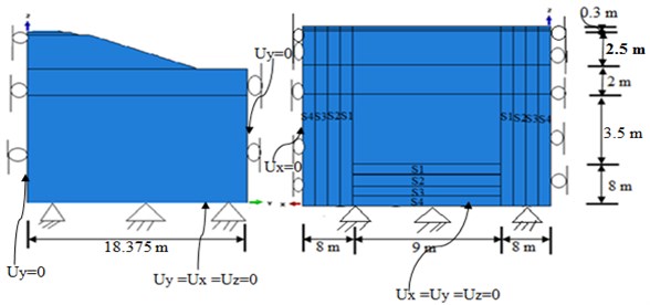
Table 2The Rayleigh damping factors α and β for different sections
Section name | (1/s) | (s) |
S1 | 2.5 | 0.3 |
S2 | 5 | 0.7 |
S3 | 15 | 1.5 |
S4 | 20 | 2 |
Fig. 9The contour plot of total velocity in: a) the original model, b) the model with artificial non-reflecting boundary at t= 0.2 s
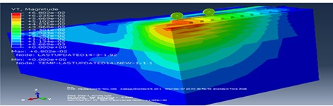
a)
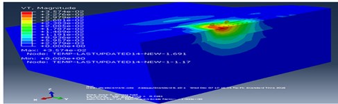
b)
3. Validation of the computational model
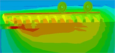
Ground vibrations induced from railway track and other random dynamic overload accounts for inertial effects, damping and time dependent load all require nonlinear dynamic analysis because the model may exhibit large displacement (non-linear geometry), especially to the presence of soft soils. In order to consider all these effects, the powerful computational finite element Package ABAQUS is used for dynamic analysis.
However, there are no direct validations of the predictions against practical measurements. Only comparisons are taken out with the published Thack et al work [3], which is used finite element package ABAQUS, and verified by Krylov’s analytical solution. The geometry, parameters and locations used for verifications are shown in [3]. Fig. 10(a) and Fig. 10(b), proved that the computational model can simulate the investigation with excellent accuracy, since the vertical displacement at three locations transversely spaced out the rail o m, 5 m and 10 m due to the passage of the wheel-set is similar in shape, timing and magnitude. Note that the main focus of this study is to compare the peak responses obtained by different choice of parameters.
Fig. 10Comparison between: a) modeling result [3], b) modeling result of this paper
![Comparison between: a) modeling result [3], b) modeling result of this paper](https://static-01.extrica.com/articles/18725/18725-img19.jpg)
a)
![Comparison between: a) modeling result [3], b) modeling result of this paper](https://static-01.extrica.com/articles/18725/18725-img20.jpg)
b)
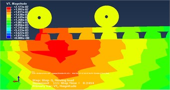
4. Response evaluations
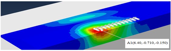
Ground vibrations for engineering purposes are usually quantified in terms of Peak Particle Velocity (PPV) [19]. PPV can be defined in several different ways, one of these are peak vertical value (VZ, Max), since the peak particle velocities in three mutually perpendicular directions, may not occur simultaneously [20]. Besides, the table of participation factor for the modal analysis indicated that the embankment railway starts vibrating predominately in the vertical direction. Therefore, to study the dynamic effect of the sub-grade soil conditions, comparisons on the Peak Vertical Velocity (PVV) are made based on the predicated result by varying material parameters. The analysis has been analyzed in time domain at A1 (at the surface of the sub-grade) due to moving of train loads.
Fig. 11Evaluation point
5. Results and discussions
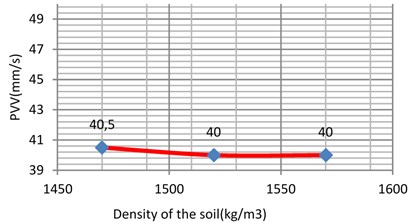
5.1. The effect of varying the unit weight of the soil
The unit weight was varied between two reasonable and expected values. For example, from 1330 kg/m3 to 1500 kg/m3 for soft clay 1470 kg/m3 to 1570 kg/m3 for loose sand 1730 kg/m3 to 1900 kg/m3 for the stiff clay and 1800 kg/m3 to 2000 kg/m3 for the dense sand i.e. in step of 50-100 kg/m3. As the results shown in Fig. 12-14 and 15, it can be concluded that unit weight has a minor influence on the response of the model with the PVV only varying to 1.62 %, 4.16 %, 1.2 % and 4.25 % for the soft clay, stiff clay, loose sand and dense sand, respectively.
Fig. 12Vibration levels in the evaluation point A1 for different density of the sub-grade (soft clay)
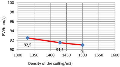
Fig. 13Vibration levels in the control point A1 for different density of the sub-grade (loose sand)
5.2. The effect of varying the Young’s modulus of the soil
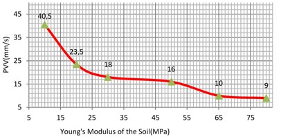
The Young’s modulus of the soil may have different values and was varied between 10 MPa to 30 MPa for loose sand and 50 MPa to 80 MPa for dense uniform sand. In addition, the Young’s modulus of the soft clay varied between 2.5 MPa to 8 MPa and 15 MPa to 40 MPa for the stiff clay [4].
Fig. 14Vibration levels in the evaluation point A1 for different density of the sub-grade (stiff clay)
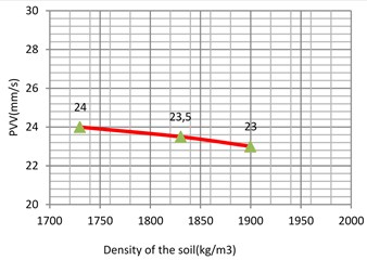
Fig. 15Vibration levels in the evaluation point A1 for different density of the sub-grade (dense sand)
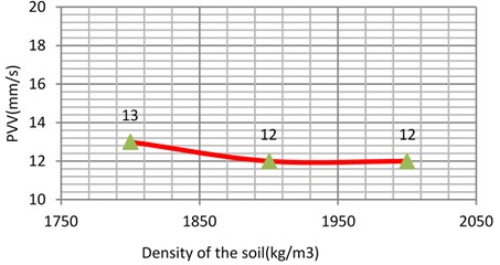
Fig. 16Vibration levels in the evaluation point A1 for different Young’s modulus of the sub-grade (clay)
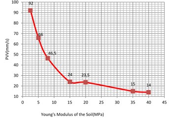
Fig. 17Vibration levels in the evaluation point A1 for different Young’s modulus of the sub-grade (sand)
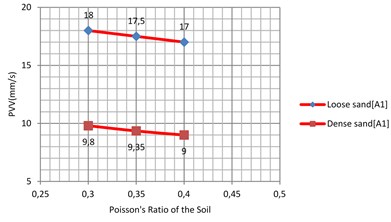
5.3. The effect of varying the Poisson’s ratio of the soil
The Poisson’s ratio of the soil was varied between 0.1 to 0.3 for clay soil and 0.3 to 0.4 for commonly used sand soil [21]. Results are shown in Fig. 18 and Fig. 19. Similar to the effect of the density, the Poisson’s ratio of the sub-grade shows only small influence on the PVV. An approximate variation of 6.93 % for the soft clay and 12 % for the stiff clay was observed. Similarly, the PVV variation for the loose sand and dense is calculated as 5.56 % and 8.16 %, respectively.
Fig. 18Vibration levels in the evaluation point A1 for different Poisson’s ratio of the sub-grade (soft and stiff clay)
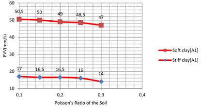
Fig. 19Vibration levels in the evaluation point A1 for different Poisson’s ratio of the sub-grade (loose and dense sand)
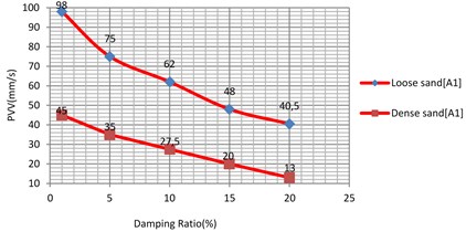
5.4. The effect of varying the damping ratio of the soil
The analyses were performed for the damping ratio of sub-grade as 1 %; 5 %; 10 %; 15 %; 20 % and comparison for similar soil type are made.
When compared with the other parameters, soil damping does have very high influence on the vibration levels of all soil types. Fig. 20 and 21, show that the variation of PVV for 1 % and 20 % is rounded to 42.5 %, 58.6 %, 60.66 % and 71.11 % for the soft clay, loose sand, stiff clay, dense sand, respectively.
Fig. 20Vibration levels in the evaluation point A1 for different damping ratio of the sub-grade (soft and stiff clay)
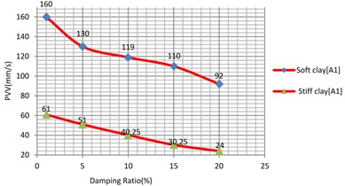
Fig. 21Vibration levels in the Evaluation point A1 for different damping ratio of the sub-grade (loose and dense sand)
6. Conclusions
This study consists of dynamic analysis of embankment railway project using finite element package ABAQUS. The effect of four group of sub-grade parameters; including the unit weight, Young’s modulus, Poisson’s ratio and the damping ratio on the maximum value of vertical velocity were investigated.
Based on the results of parametric study, it can be concluded that the Young’s modulus has quite significant effect on the surface vibration levels. Meanwhile, low Young’s modulus of the sub-grade material, can result in a large amplification of the surface vibrations within the railway track, i.e. a Young’s modulus of 35 MPa for clay and 65 MPa for sand soil is deemed most efficient in minimizing the vibration induced at the railway track. Moreover, it is found that the damping ratio of the sub-grade has much greater influence on the surface vibration levels than the Young’s modulus. Conversely, the effects of both unit weight and Poisson’s ratio on the surface vibrations are insignificant compared to the effect of Young’s modulus and damping ratio. Hence to fulfill the technical requirement of the railway track, special attention regarding to the Young's modulus and the damping ratio of the sub-grade should be paid.
References
-
Galvin P., Dominguez J. Experimental and numerical analyses of vibrations induced by high-speed trains on the Cordoba-Malaga line. Soil Dynamics and Earthquake Engineering, Vol. 29, Issue 4, 2009, p. 641-657.
-
Fuggini C., Zangani D. Numerical Investigation of the Effect of Variable Subsoil Conditions and Freight Traffic on Railway Infrastructure. Transport Research Arena, Paris, 2014.
-
Thack P. N., Kongo G. Q. A prediction model for train-induced track vibrations. Electronic Journal of Geotechnical Engineering, Vol. 17, 2012, p. 3559-3569.
-
Hasna P. H. Study of dynamic behavior of rail track using finite element method. International Journal of Engineering Research and General science, Vol. 3, Issue 6, 2015, p. 668-676.
-
Connolly D., Giannopoulos A., Forde M. C. Numerical modelling of ground borne vibrations from high speed rail lines on embankments. Soil Dynamics and Earthquake Engineering, Vol. 46, 2013, p. 13-19.
-
Fu Q., Zheng C. Three-dimensional dynamic analyses of track-embankment-ground system subjected to high speed train loads. The Scientific World Journal, 2014, p. 924592.
-
Madshus C., Bessason B., Harvik L. Prediction model for low frequency vibration from high speed railways on soft ground. Journal of Sound and Vibration, Vol. 193, Issue 1, 1996, p. 195-203.
-
Dahlberg T. T. Handbook of Railway Dynamics. CRC Press, London, 2006.
-
Kumaran G., Menon D., Nair K. K. Dynamic studies of rail track sleepers in track structures system. Journal of Sound and Vibration, Vol. 15, Issue 4, 2003, p. 485-501.
-
Kerr A. Fundamentals of Railway Track Engineering. Simmons-Boardman Books, 2003.
-
Montero J. N. Vibration Analysis of Underground Tunnel at High-Tech Facility. Department of Construction Sciences, Sweden, August 2010.
-
Serdaroglu M. S. Non-linear Analysis of Pile driving and Ground Vibrations in Saturated Cohesive Soils Using FEM. Ph.D. Thesis, University of Iowa, 2010.
-
ABAQUS Analysis User’s Manual. Version 6.13, Dassault Systemes Simulia Corp., 2013.
-
Durgunoglu H. T., Mitchell J. K. Static penetration resistance of soils: I. Analysis. Proceeding of the Conference on In Situ Measurement of Soil Properties, ASCE, New York, 1975, p. 151-171.
-
Durgunoglu H. T., Mitchell J. K. Static penetration resistance of soils: II. Evaluation of theory and implication for practice. Proceeding of the Conference on In Situ Measurement of Soil Properties, ASCE, New York, 1975, p. 172-189.
-
Susila E., Hrychiw R. D. FEM modelling of the cone penetration test (CPT) in normally consolidated sand. International Journal for Numerical and Analytical Methods in Geomechanics, Vol. 27, 2003, p. 585-602.
-
Coefficients of Friction. Wikipidia.org.
-
Yun Z. Finite Element Analysis of Vibration Excited by Rail-Wheel Interaction. Master’s Thesis, University of Hong Kong, 2014.
-
Deckner F. Ground Vibrations Due to Pile and Sheet Pile Driving. Licentiate of Thesis, Royal Institute of Technology, Stockholm, Sweden, 2013.
-
Head J. M., Jardine F. M. Ground-Borne Vibrations Arising from Piling. Ciria Technical Note 142, CIRIA, London, U.K, 1992.
-
Bowles J. E. Foundation Analysis and Design. 5th Edition, McGraw-Hill Higher Education, 2001.
About this article

The work was carried out at the school of civil engineering, University of Mekelle, Ethiopian Institute of Technology-Mekelle. The authors acknowledge the provision of valuable discussions with Abdulziz Osman, Assistant professor at Ethiopian Institute of Technology-Mekelle, Mekelle, Tigray, Ethiopia, Argaw Asha (Ph. D), Director of Ethiopian Institute of Construction, Addis Ababa, Ethiopia, and Ahmed Mohamed (Ph. D), Assistant professor at Ethiopian Institute of Technology – Mekelle, Mekelle, Tigray, Ethiopia. Financial supports were provided by Ethiopia Roads Authority and University of Mekelle.
