Numerical investigation on nonlinear dynamic responses to fluid-structure interaction in BTA deep-hole drilling shaft system

Ma, Guohong; Shen, Xingquan

doi:10.21595/jve.2017.18691

Journal of Vibroengineering

Browse Journal

Submit article

Published: 15 November 2017

Check for updates

Numerical investigation on nonlinear dynamic responses to fluid-structure interaction in BTA deep-hole drilling shaft system

Guohong Ma¹

Xingquan Shen²

¹School of Mechanical and Power Engineering, North University of China, Taiyuan, People’s Republic of China

²Taiyuan University of Technology, Taiyuan, People’s Republic of China

Corresponding Author:

Guohong Ma

Cite the article Download PDF

Downloads 1545

WoS Core Citations 1

Abstract

Numerical investigation is conducted into the nonlinear dynamic responses to fluid-structure interaction in deep-hole drilling shaft system. Based on the theories of pipes and tubes conveying fluid, the governing equation of the drilling shaft system is obtained taking into account of the fluid-structure interaction and the effect of the motion constraints. The nonlinear partial differential governing equation of motion is discretized in modal space using the Galerkin method and then transformed into a set of ordinary different equations. Numerical solutions of these equations are then obtained using the fourth order Runge-Kutta method. The influence of the forcing frequency and the support constraints on the dynamic behaviors of the drilling shaft is examined. The nonlinear dynamic behaviors of the drilling shaft system are presented by the bifurcation diagram and phase diagram. It has been found that the magnitude of support stiffness and the number and position of support constraints have a significant influence on dynamic behaviors of the drilling shaft system. The study in the paper provides an effective guidance to maintain the stability of the BTA deep-hole drilling shaft system through selecting the favorable operation parameters in deep hole drilling process.

1. Introduction

The deep-hole drilling shaft system is a complex system with internal interaction. It is difficult to predict and control such nonlinear dynamic behaviors as whirling vibration, tool chatter and cutting fluid disturbance, which result in an adverse effect on processing quality in deep-hole drilling process [1-5].

Recently, great importance has been attached to investigate the dynamic characteristics of the drilling shaft system in the deep hole drilling process. Chin [6, 7] established the three-dimensional general equations for lateral, longitudinal and torsional motion of the shaft containing the fluid flow to investigate the deep-hole drilling shaft eigen properties based on the Euler beam theory. Kong [8, 9] constructed the dynamic model for rotating drilling shaft with multi-span supports using lots of 2-nodeTimoshenko beam element model with free-interface to investigate the nonlinear dynamic responses considering the effects of the mass eccentricity and the cutting force fluctuating and in addition, presented a modified Newton shooting method to obtain the periodic trajectories of the dynamic system and analyze the periodic dynamic behaviors of the drilling shaft system. Perng [10] developed equations of motion for two different models: a Timoshenko beam model and a Euler-Bernoulli beam model. He analyzed the eigen properties of spinning boring trepanning association (BTA) deep-hole drilling shaft containing flowing fluid and subject to compressive axial force. Ahmadi [11] presented a generalized stability model for drilling dynamics considering the regeneration of chip thickness due to the tool deflection in the lateral, torsional and axial directions. Al-Wedyan [12] presented an approach to investigate the whirling motion of the BTA deep hole drilling system by introducing the system excitation in the form of internal forces between the drilling shaft and the workpiece. Matsuzaki [13] proposed an analytical model to study chatter vibration considering the support position of the drilling shaft in detail such as at the oil pressure head, the supporting pad and the base, and investigated numerically the stability of the self-excited vibration.

The nonlinear vibrations of supported pipes conveying fluid have been studied before by other researchers [14-17]. Wang [18, 19] investigated the nonlinear dynamics of simply supported pipes conveying pulsating fluid with non-linear motion constraints. However, nonlinear dynamic behaviors of pipes conveying fluid with multi-span intermediate supports have rarely been discussed. At present, there are significant differences between the theoretically simplified model and the actual process situation with regard to the research of the dynamic behavior of the deep hole drilling shaft system. Moreover, most of the proposed models are biased in the one-way analysis, whereas the interaction is complex in the deep hole drilling system. Therefore, it is necessary to establish the interaction model to study the interaction effect and provide theoretical guidance for the actual drilling process.

In this paper, the fluid-structure interaction model is established to investigate the nonlinear dynamic characteristics of fluid-structure interaction of the deep hole drilling shaft system. The effect of the motion constraints on the drilling shaft is discussed in detail when the situation of the drilling shaft supported by the auxiliary support and the oil pressure head is divided into four cases. The rich and complex nonlinear dynamic behaviors of the drilling shaft system are showed by the bifurcation diagram and phase diagram.

2. The equation of motion

In the drilling shaft system, the drilling shaft is fed in the axial direction while the workpiece rotates. The drilling shaft behavior of the BTA drill is investigated in transient state of the deep hole drilling process. As shown in Fig. 1, the drilling shaft is modeled as a Euler-Bernoulli beam which is clamping at one end and hinging at the other end [10].

Fig. 1Schematic diagram of the drilling shaft system

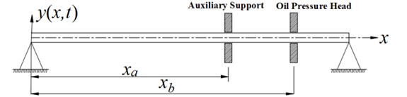
Based on the theories of pipes and tubes conveying fluid, the governing equation of the drilling shaft system for lateral vibration is established taking into account of the interaction between the drilling shaft and the cutting fluid, and the effect of the motion constraints of the auxiliary support and the oil pressure head on the drilling shaft. The motion constraints of the auxiliary support and the oil pressure head is assumed to be linear springs. The equation of motion [18] is given by:

1

\begin{array}{l} \begin{array}{l} (M + m) \frac{\partial^{2} y}{\partial t^{2}} + 2 M U \frac{\partial^{2} y}{\partial x \partial t} + [\begin{matrix} M U^{2} + M \frac{\partial U}{\partial t} (l - x) \\ - (1 + a \frac{\partial}{\partial t}) \frac{E A}{2 I} \int_{0}^{1} {(\frac{\partial y}{\partial x})}^{2} d x \end{matrix}] \frac{\partial^{2} y}{\partial x^{2}} + (1 + a \frac{\partial}{\partial t}) E I \frac{\partial^{4} y}{\partial x^{4}} \\ + K_{1} y δ (x - x_{a}) + K_{2} y δ (x - x_{b}) = 0, \end{array} \end{array}

where $M$ is mass of the cutting fluid per unit length. $m$ is mass of the drilling shaft per unit length. $U$ represents flow velocity of the cutting fluid. $A$ is the cross sectional area of the drilling shaft. $I$ is the moment of inertia of the cross sectional area. $l$ is the length of the drilling shaft. $E$ is Young’s modulus of the drilling shaft. $a$ is viscoelastic damping coefficient. $x_{a}$ and $x_{b}$ are the distance from the origin along the central axis line of the drilling shaft. $K_{1}$ and $K_{2}$ are the support stiffness at the position of $x_{a}$ and $x_{b}$ , respectively. $x$ is the coordinate along the central axis line of the drilling shaft. $t$ is the time. $y (x, t)$ is the transverse displacement function of $x$ and $t$ . $δ$ is the Dirac delta function.

It is convenient to introduce the dimensionless quantities as follows:

η = \frac{y}{l}, ξ = \frac{x}{l}, τ = {(\frac{E I}{M + m})}^{1 / 2} \frac{t}{l^{2}}, u = {(\frac{M}{E I})}^{1 / 2} U l, β = \frac{M}{M + m}, k = \frac{A l^{2}}{2 I},

α = {(\frac{E I}{M + m})}^{1 / 2} \frac{a}{l^{2}}, ξ_{a} = \frac{x_{a}}{l}, ξ_{b} = \frac{x_{b}}{l}, k_{1} = \frac{K_{1} l^{3}}{E I}, k_{2} = \frac{K_{2} l^{3}}{E I} .

And the equation is rearranged as:

2

\begin{array}{l} \begin{array}{l} α \frac{\partial^{5} η}{\partial ξ^{4} \partial τ} + \frac{\partial^{4} η}{\partial ξ^{4}} + [u^{2} + \sqrt{β} \frac{\partial u}{\partial τ} (1 - ξ)] \frac{\partial^{2} η}{\partial ξ^{2}} + 2 \sqrt{β} u \frac{\partial^{2} η}{\partial ξ \partial τ} + \frac{\partial^{2} η}{\partial τ^{2}} - k \frac{\partial^{2} η}{\partial ξ^{2}} {\int_{0}^{1} (\frac{\partial η}{\partial ξ})}^{2} d ξ \\ - 2 α k \frac{\partial^{2} η}{\partial ξ^{2}} \int_{0}^{1} \frac{\partial η}{\partial ξ} \frac{\partial^{2} η}{\partial ξ \partial τ} d ξ + k_{1} η δ (ξ - ξ_{a}) + k_{2} η δ (ξ - ξ_{b}) = 0 . \end{array} \end{array}

The cutting fluid velocity in the drilling shaft is assumed to be harmonically fluctuating and the dimensionless flow velocity $u$ is defined as:

3

u = u_{0} (1 + μ s i n ω τ),

where $μ$ and $ω$ represents the perturbation amplitude and forcing frequency, respectively; $u_{0}$ is the mean flow velocity.

3. Method of solution

The solutions of the dimensionless non-linear partial differential equation are discretized to the time and position functions using the Galerkin method. It is assumed that the non-dimensional displacement at any point $ξ$ can be expressed as:

4

η (ξ, τ) = \sum_{i = 1}^{N} ϕ_{i} (ξ) q_{i} (τ),

where $q_{i} (τ)$ represents the unknown time-dependent generalized coordinates and $ϕ_{i} (ξ)$ is the corresponding orthogonal eigenfunction of the beam, which is assumed to be fixed at one end and simply supported at the other end, given by:

5

ϕ_{i} (ξ) = c o s λ_{i} ξ - c o s h λ_{i} ξ - σ_{i} (s i n λ_{i} ξ - s i n h λ_{i} ξ),

σ_{i} = \frac{c o s λ_{i} + c o s h λ_{i}}{s i n λ_{i} + s i n h λ_{i}},

where the eigenvalues $λ_{i}$ are the solution of the transcendental equation:

6

t a n λ_{i} = t a n h λ_{i} .

In this study, the series Eq. (4) is truncated at $N =$ 10.

Thus, the first ten values of $λ_{i}$ that satisfy the above Eq. (6) are shown in Table 1.

Table 1The value of λi

$λ_{i}$	Value of $λ_{i}$	$λ_{i}$	Value of $λ_{i}$
$λ_{1}$	3.92660246	$λ_{6}$	19.63495408
$λ_{2}$	7.06858275	$λ_{7}$	22.77654674
$λ_{3}$	10.21017612	$λ_{8}$	25.91813939
$λ_{4}$	13.35176878	$λ_{9}$	29.05973205
$λ_{5}$	16.49336143	$λ_{10}$	32.20132470

Substituting Eq. (4) into Eq. (2), multiplying both sides of Eq. (2) by the $j$ th eigenfuction $ϕ_{j} (ξ)$ and integrating from 0 and 1, the following equation in matrix form can be obtained:

7

\ddot{q} + C \dot{q} + K q + H + F = 0,

where $C$ and $K$ are $N \times N$ matrices, and $q$ , $H$ and $F$ are $N \times 1$ matrices. They can be defined as:

q = (q_{1}, q_{2}, \dots, q_{N})^{T},

C = B_{0}^{- 1} \{α B_{3} + 2 \sqrt{β} u B_{1}\},

K = B_{^{0}}^{- 1} \{B_{3} + u^{2} B_{2} + (\sqrt{β} μ u_{0} ω c o s ω τ) (B_{2} - B_{4})\},

H = B_{0}^{- 1} \{- k q^{T} B_{5} q B_{2} q - 2 α k q^{T} B_{5} \dot{q} B_{2} q\},

F = B_{0}^{- 1} \{F 1 + F 2\} = B_{0}^{- 1} \{k_{1} [\begin{array}{l} (\sum_{i = 1}^{N} ϕ_{i} (ξ_{a}) q_{i}) ϕ_{1} (ξ_{a}) \\ (\sum_{i = 1}^{N} ϕ_{i} (ξ_{a}) q_{i}) ϕ_{2} (ξ_{a}) \end{array}] + k_{2} [\begin{array}{l} (\sum_{i = 1}^{N} ϕ_{i} (ξ_{b}) q_{i}) ϕ_{1} (ξ_{b}) \\ (\sum_{i = 1}^{N} ϕ_{i} (ξ_{b}) q_{i}) ϕ_{2} (ξ_{b}) \end{array}]\} .

And the elements of $B_{0}$ through $B_{5}$ are shown as follows:

B_{0} (i, j) = \int_{0}^{1} ϕ_{i} (ξ) ϕ_{j} (ξ) d ξ, B_{1} (i, j) = \int_{0}^{1} ϕ_{i} (ξ) ϕ_{j}^{'} (ξ) d ξ,

B_{2} (i, j) = \int_{0}^{1} ϕ_{i} (ξ) ϕ_{j}^{''} (ξ) d ξ, B_{3} (i, j) = \int_{0}^{1} ϕ_{i} (ξ) ϕ_{j}^{(4)} (ξ) d ξ,

B_{4} (i, j) = \int_{0}^{1} ξ ϕ_{i} (ξ) ϕ_{j}^{''} (ξ) d ξ, B_{5} (i, j) = \int_{0}^{1} ϕ_{i}^{'} (ξ) ϕ_{j}^{'} (ξ) d ξ,

where $i$ , $j$ represents the $i$ th row and the $j$ th column of the matrix, respectively.

To solve it simply, the state vector is introduced as follows:

8

Z = \{\begin{array}{l} q \\ \dot{q} \end{array}\} .

Thus, Eq. (7) is transformed into its first-order form:

9

\dot{Z} = A Z + D + G,

where $A$ is $2 N \times 2 N$ matrices and $D$ and $G$ are $2 N \times 1$ matrices. They can be defined as:

A = [\begin{matrix} S & T \\ - K & - C \end{matrix}], D = [\begin{matrix} Q \\ - H \end{matrix}], G = [\begin{matrix} Q \\ - F \end{matrix}], S = O_{N \times N}, T = I_{N}, Q = O_{N \times 1} .

4. Numerical results and discussion

In order to study the effect of support constraints on the vibration of the drilling shaft system, the support conditions are divided into the following four cases: (1) In the case of $k_{1} =$ 0 and $k_{2} =$ 0, the drilling shaft system is without support constraints. (2) In the case of $k_{1} \neq$ 0 and $k_{2} =$ 0, the shaft system is only supported at the position of $ξ_{a}$ . (3) In the case of $k_{1} =$ 0 and $k_{2} \neq$ 0, the drilling shaft system is only supported at the position of $ξ_{b}$ . (4) In the case of $k_{1} \neq$ 0 and $k_{2} \neq 0$ , the drilling shaft system is supported at the position of $ξ_{a}$ and $ξ_{b}$ at the same time.

The parameters of the drilling shaft system are listed in Table 2. In the study, letting the dimensionless quantity $α =$ 0.0005, $u_{0} =$ 3.5, $μ =$ 0.4, $ξ_{a} =$ 0.6 and $ξ_{b} =$ 0.8, respectively.

Table 2The parameters of the drilling shaft system

Young’s modulus $E$ (Pa)	Density of the drilling shaft $ρ_{z}$ (kg/m³)	Density of the cutting fluid $ρ_{f}$ (kg/m³)	Internal diameter $d_{1}$ (mm)	External diameter $d_{2}$ (mm)	Length $l$ (m)
2.14×10¹¹	7.8×10³	0.865×10³	20	26	5

The numerical solutions of Eq. (9) are obtained by the fourth order Runge-Kutta method.

The displacement and velocity of the midpoint of the drilling shaft are given by:

10

η (0.5, τ) ≅ \sum_{i = 1}^{N} ϕ_{i} (0.5) z_{i} (τ), \dot{η} (0.5, τ) ≅ \sum_{i = 1}^{N} ϕ_{i} (0.5) z_{i + N} (τ) .

4.1. Vibration characteristics of the drilling shaft without support constraints

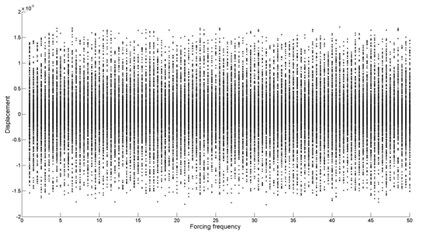
Fig. 2 is the bifurcation diagram of the drilling shaft system with forcing frequency. The abscissa is the forcing frequency and the ordinate represents the lateral vibration displacement of the midpoint of the drilling shaft. In the calculations to construct the bifurcation diagram, the initial vibration process of the drilling shaft is omitted and only the situation is recorded when the drilling shaft vibration is relatively stable. whenever the vibration velocity at the position of $ξ =$ 0.5 tends to zero from positive or negative $(\dot{η} (0.5, τ) ≅ \sum_{i = 1}^{N} ϕ_{i} (0.5) z_{i + N} (τ) \to 0),$ the midpoint displacement at that time is recorded. Thus, the vibration displacement contains positive and negative values in the bifurcation diagram.

Fig. 2Bifurcation diagram of the drilling shaft with forcing frequency for k1= 0 and k2= 0

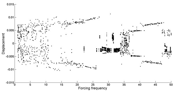
As shown in Fig. 2, it can be found that, with the increasing of the forcing frequency, the drilling shaft system shows extremely rich dynamical behaviors, such as a variety of forms of periodic motions, quasi-periodic motion and chaotic motion.

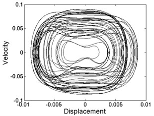
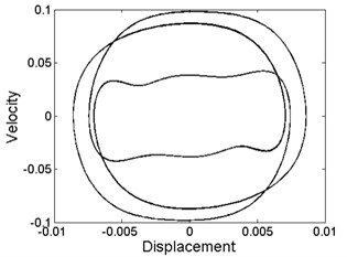
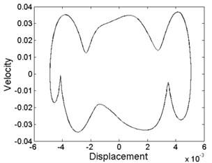
Fig. 3Phase diagram of different levels of forcing frequency: a) ω= 10.8, phase-chaos, b) ω= 13.6, period-1 motion, c) ω= 20, period-3 motion, d) ω= 28.2, period-4 motion, e) ω= 36.8, quasi-periodic motion, f) ω= 39.6, quasi-periodic motion, g) ω= 40.8, period-2 motion, h) ω= 48.6, period-1 motion

Phase diagram of different levels of forcing frequency: a) ω= 10.8, phase-chaos, b) ω= 13.6, period-1 motion, c) ω= 20, period-3 motion, d) ω= 28.2, period-4 motion, e) ω= 36.8, quasi-periodic motion, f) ω= 39.6, quasi-periodic motion, g) ω= 40.8, period-2 motion, h) ω= 48.6, period-1 motion

a)

b)

c)

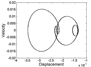
d)

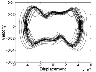
e)

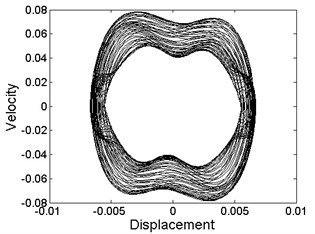
f)

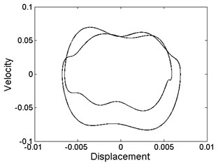
g)

h)

As can be seen from Fig. 3, quasi-periodic motion and chaotic motion can be observed in most of the regions of $1 < ω < 11.5$ , $27 < ω < 37.5$ and $47.5 < ω < 50$ , where a few of the periodic motions are hidden as illustrated in Fig. 3(h).

However, the periodic motion mainly appears in the other regions. Of course, these regions contain a minority of the quasi-periodic motion and chaotic motion as shown in Fig. 3(f).

4.2. Effect of support constraints at the position of $ξ_{a}$ on the vibration of the drilling shaft

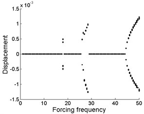
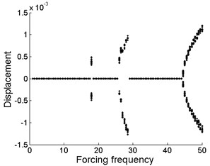
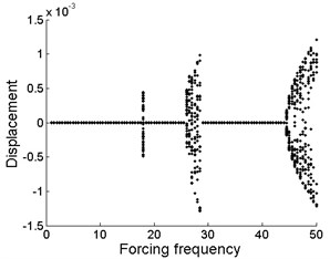
In this case, the drilling shaft is restrained by support constraints at the position of $ξ_{a}$ . From Fig. 4(a), (b) and (c), it is found that the common feature of the three is that the stable motion almost appears in the same regions such as $1 < ω < 18$ , $18 < ω < 26$ and $28.5 < ω < 44.5$ for different values of support stiffness $k_{1}$ . The emergence of local stable regions of the system is due to the support constraints at the position of $ξ_{a}$ . In addition, there exists three bifurcation starting points, which are at the forcing frequency of $ω =$ 18, $ω =$ 26 and $ω =$ 44.5, respectively. The bifurcation region is expanded with the increase of the forcing frequency.

However, the motion form of the drilling shaft system is different in the bifurcation regions for different levels of support stiffness $k_{1}$ . Periodic motion appears, as shown in Fig. 4(a). The drilling shaft system undergoes periodic motion, as can be seen in Fig. 4(b). Chaotic motion occurs, as can be found in Fig. 4(c).

In the absence of support constraints, the system always presents nonlinear characteristics, as shown in Fig. 2. After the linear constraints is imposed to the drilling shaft, the nonlinear characteristics of the system is obviously improved. Chaotic and quasi-periodic motion rarely appear, and most importantly, stable motion appears. With the increase of forcing frequency, restabilization is repeatedly detected in Fig. 4. This indicates that linear constraints plays a key role in the dynamic characteristics of nonlinear system. Linearity of the linear constraints itself has been incorporated into the nonlinear system. Thus, the system contains both linear and nonlinear characteristic. The specific performance of the dynamic characteristics of the system depends on the forcing frequency.

Fig. 4Bifurcation diagram of the drilling shaft with forcing frequency for different levels of the support stiffness k1 at the position of ξa: a) k1= 2×105, b) k1= 2×106, c) k1= 2×107

Bifurcation diagram of the drilling shaft with forcing frequency for different levels of the support stiffness k1 at the position of ξa: a) k1= 2×105, b) k1= 2×106, c) k1= 2×107

a)

b)

c)

4.3. Effect of support constraints at the position of $ξ_{b}$ on the vibration of the drilling shaft

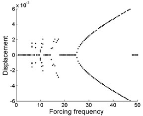
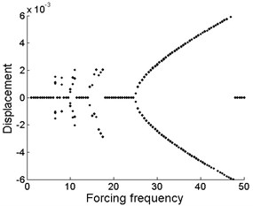
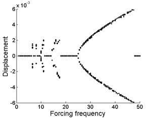
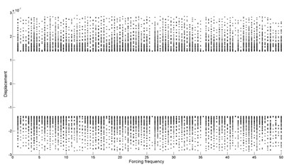
From Fig. 5(a), (b) and (c), it is obtained that the motion form is almost the same in the whole region for different values of support stiffness $k_{2}$ , which implies that the magnitude of the support stiffness $k_{2}$ at the position of $ξ_{b}$ plays little role in the vibration displacement of midpoint of the drilling shaft system. Periodic motion occurs in the bifurcation regions of $ω =$ 6.5, $ω =$ 8, $9.5 < ω < 12$ , $14 < ω < 18$ and $24.5 < ω < 48.5$ . For other forcing frequency values, the stable regions are shown in Fig. 5(a), (b) and (c), respectively. Moreover, these stable regions emerge as a result of the support constraints at the position of $ξ_{b}$ .

As shown in Fig. 5, the bifurcation diagram of the drilling shaft system is similar to that of Fig. 4. Similarly, restabilization is also repeatedly found in Fig. 5. However, the difference of the distribution and quantity of the stable regions is due to the change of the location of support constraints.

Fig. 5Bifurcation diagram of the drilling shaft with forcing frequency for different levels of the support stiffness k2 at the position of ξb: a) k2= 2×105, b) k2= 2×106, c) k2= 2×107

Bifurcation diagram of the drilling shaft with forcing frequency for different levels of the support stiffness k2 at the position of ξb: a) k2= 2×105, b) k2= 2×106, c) k2= 2×107

a)

b)

c)

4.4. Coupled effect of support constraints at the position of $ξ_{a}$ and $ξ_{b}$ on the vibration of the drilling shaft

Representative combination levels of the support stiffness $k_{1}$ and $k_{2}$ are studied. As can be seen in Fig. 6, the difference of dynamic characteristics of the system is extraordinarily obvious with respect to different combination levels of the support stiffness $k_{1}$ and $k_{2}$ .

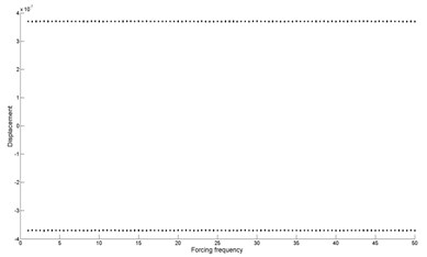
As shown in Fig. 6(a), it can be seen that the drilling shaft system undergoes periodic-1 motion. From Fig. 6(b), it is found that quasi-periodic motion and chaotic motion occur. In Fig. 6(c), the movement of the drilling shaft system is quasi-periodic motion and chaotic motion in the whole region, except for the forcing frequency $ω =$ 26 (periodic-3 motion), $ω =$ 36.5 (periodic-1 motion) and $ω =$ 41.5 (periodic-5 motion).

When single support constraints are imposed on the drilling shaft, the magnitude of the support stiffness has little effect on the dynamic characteristics of the system, as shown in Fig. 4 and Fig. 5. However, different combination levels of the support stiffness exert remarkable influence on the dynamic characteristics of the system, as can be seen in Fig. 6, when two support constraints are imposed on the drilling shaft. Moreover, the bifurcation diagram in Fig. 6 is not a linear superposition of the corresponding bifurcation diagram in Fig. 4 and Fig. 5. This indicates that there is the coupling effect due to the two linear constraints in the nonlinear system, which plays an important role in the dynamic characteristics of the system. In addition, it should be pointed out that no restabilization is found with the increasing of forcing frequency.

Fig. 6Bifurcation diagram of the drilling shaft with forcing frequency for different combination levels of the support stiffness k1 and k2 at the position of ξa and ξb: a) k1= 2×106, k2= 2×105, b) k1= 2×106, k2= 2×107, c) k1= 2×107, k2= 2×106

Bifurcation diagram of the drilling shaft with forcing frequency for different combination levels of the support stiffness k1 and k2 at the position of ξa and ξb: a) k1= 2×106, k2= 2×105, b) k1= 2×106, k2= 2×107, c) k1= 2×107, k2= 2×106

a)

b)

c)

5. Conclusions

In this investigation, the influence of the forcing frequency and support constraints on the dynamic behaviors of the drilling shaft system has been illustrated. The numerical results provide guidelines for maintaining the system stability by selecting the appropriate forcing frequency of the cutting fluid supply and the different support constraints. The following main conclusions have been drawn in this study.

Single support constraints can improve the nonlinear characteristics of the system. In the absence of support constraints, the system always presents nonlinear characteristics. After the drilling shaft is subjected to single support constraints, chaotic and quasi-periodic motion rarely appear, and most importantly, stable motion appears. In addition, restabilization is repeatedly detected.

Different combination levels of support stiffness have a significant effect on nonlinear dynamic behaviors of the system owing to the coupling effect of linear support constraints at different positions.

It ought to be pointed out that, the influence of distribution position of the support constraints on dynamic characteristics of the drilling shaft system is studied in a transient state of the drilling shaft. However, the position of the support constraints relative to the drilling shaft is variable in the drilling operations, which results in the change of the dynamic characteristics of the system. Therefore, the change of the position of the support constraints on the dynamic characteristics should be further studied.

References

Raabe N. Dynamic disturbances in BTA deep-hole drilling: modelling chatter and spiraling as regenerative of the effects. Intelligence, Studies in the Classification, Data Analysis, and Knowledge Organization, 2010, p. 745-754.

Publisher
Fuji H., Marui E., Ema S. Whirling vibration in drilling. Part 3: Vibration analysis in drilling workpiece with a pilot hole. Journal of Engineering for Industry, Vol. 110, Issue 4, 1988, p. 315-321.

Publisher
Fuji H., Marui E., Ema S. Whirling vibration in drilling. Part 2: Influence of drill geometries, particularly of the drill flank, on the initiation of vibration. American Society of Mechanical Engineer. Production Engineering Division, Vol. 13, 1984, p. 323-331.

Search CrossRef
Mehrabadi I. M., Nouri M., Madoliat R. Investigating chatter vibration in deep drilling, including process damping and the gyroscopic effect. International Journal of Machine Tools and Manufacture, Vol. 49, Issues 12-13, 2009, p. 939-946.

Publisher
Bayly P. V., Lamar M. T., Calvert S. G. Low-frequency regenerative vibration and formation of lobed holes in drilling. Journal of Manufacturing Science and Engineering Transactions of the ASME, Vol. 124, Issue 2, 2002, p. 275-285.

Publisher
Chin J. H., Lee L. W. A study on the tool eigenproperties of a BTA deep hole drill theory and experiments. International Journal of Machine Tools and Manufacture, Vol. 35, Issue 1, 1995, p. 29-49.

Publisher
Chin J. H., Hsieh C. T., Lee L. W. The shaft behavior of BTA deep hole drilling tool. International Journal of Mechanical Sciences, Vol. 38, Issue 5, 1996, p. 461-482.

Publisher
Kong L. F., Li Y., Lu Y. J. Complex nonlinear behaviors of drilling shaft system in boring and trepanning association deep hole drilling. International Journal of Advanced Manufacturing Technology, Vol. 45, Issues 3-4, 2009, p. 211-218.

Publisher
Kong L. F., Li Y., Zhao Z. Y. Numerical investigating nonlinear dynamic responses to rotating deep-hole drilling shaft with multi-span intermediate supports. International Journal of Non-Linear Mechanics, Vol. 55, 2013, p. 170-179.

Publisher
Perng Y. L., Chin J. H. Theoretical and experimental investigations on the spinning BTA deep-hole drill shafts containing fluids and subject to axial forces. International Journal of Mechanical Sciences, Vol. 41, Issue 11, 2001, p. 1301-1322.

Publisher
Ahmadi K., Altintas Y. Stability of lateral, torsional and axial vibrations in drilling. International Journal of Machine Tools and Manufacture, Vol. 68, 2013, p. 63-74.

Publisher
Al Wedyan H.-M., Bhat R. B., Demirli K. Whirling Vibrations in Boring Trepanning Association Deep Hole Boring Process: Analytical and Experimental Investigations. Journal of Manufacturing Science and Engineering Transactions of the ASME, Vol. 129, Issue 1, 2007, p. 48-62.

Publisher
Matsuzaki K., Ryu T., Sueoka A. Theoretical and experimental study on rifling mark generating phenomena in BTA deep hole drilling process. International Journal of Machine Tools and Manufacture, Vol. 88, 2015, p. 194-205.

Publisher
Panda L. N., Kar R. C. Nonlinear dynamics of a pipe conveying pulsating fluid with parametric and internal resonances. Nonlinear Dynamics, Vol. 49, Issues 1-2, 2007, p. 9-30.

Publisher
Panda L. N., Kar R. C. Nonlinear dynamics of a pipe conveying pulsating fluid with combination, principal parameter and internal resonances. Journal of Sound and Vibration, Vol. 309, Issues 3-5, 2008, p. 375-406.

Publisher
Modarres Sadeghi Y., Paidoussis M. P. Nonlinear dynamic of extensible fluid-conveying pipe, supported at both ends. Journal of Fluids and Structures, Vol. 25, Issue 3, 2009, p. 535-543.

Publisher
Giacobbi D. B., Rinaldi S., Semler C. The dynamics of a cantilevered pipe aspirating fluid studied by experimental, numerical and analytical methods. Journal of Fluids and Structures, Vol. 30, 2012, p. 73-96.

Publisher
Wang L. A further study on the non-linear dynamic of simply supported pipes conveying pulsating fluid. International Journal of Non-linear Mechanics, Vol. 44, Issue 1, 2009, p. 115-121.

Publisher
Wang L. Erratum to a further study on the non-linear dynamic of simply supported pipes conveying pulsating fluid. International Journal of Non-linear Mechanics, Vol. 45, Issue 3, 2010, p. 331-335.

Publisher

About this article

Received

29 May 2017

Accepted

31 August 2017

Published

15 November 2017

SUBJECTS

Flow induced structural vibrations

DOI

https://doi.org/10.21595/jve.2017.18691

Keywords

nonlinear dynamic behaviors

fluid-structure interaction

Galerkin method

deep hole drilling

Acknowledgements

This work was financially supported by the National Natural Science Foundation of China (51175482) and International S&T Cooperation Program of China (2013DFA70770).

This is an open access article distributed under the Creative Commons Attribution License, which permits unrestricted use, distribution, and reproduction in any medium, provided the original work is properly cited.

Previous article in issue Previous Next article in issue Next

Research article

2021 06 28

Modeling of chatter vibrations in gun drilling process

Sergey Voronov, Ivan Pleshcheev

Research article

2017 12 01

Transient vibration analysis of BTA deep-hole drilling shaft system

Guohong Ma, Xingquan Shen

Research article

2017 03 31

Numerical investigation on the propulsive performance of flexible flapping fins using CFD/CSD method

Long Liu, Haisong Ang

Research article

2016 12 31

Analytical model for nonlinear vibration of flexible rotor system

Min Wu, Shengbo Yang, Dongjiang Han, Daren Yu, Jinfu Yang

G. Ma and X. Shen, “Numerical investigation on nonlinear dynamic responses to fluid-structure interaction in BTA deep-hole drilling shaft system,” Journal of Vibroengineering, Vol. 19, No. 7, pp. 5462–5472, Nov. 2017, https://doi.org/10.21595/jve.2017.18691

Copy Extrica

Copied to clipboard!

TY  - JOUR
DO  - 10.21595/jve.2017.18691
UR  - https://doi.org/10.21595/jve.2017.18691
TI  - Numerical investigation on nonlinear dynamic responses to fluid-structure interaction in BTA deep-hole drilling shaft system
T2  - Journal of Vibroengineering
AU  - Ma, Guohong
AU  - Shen, Xingquan
PY  - 2017
DA  - 2017/11/15
PB  - JVE International Ltd.
SP  - 5462-5472
IS  - 7
VL  - 19
SN  - 1392-8716
ER  - 

Copy Ris

Copied to clipboard!

@article{Ma_2017,
	doi = {10.21595/jve.2017.18691},
	url = {https://doi.org/10.21595/jve.2017.18691},
	year = 2017,
	month = {nov},
	publisher = {{JVE} International Ltd.},
	volume = {19},
	number = {7},
	pages = {5462--5472},
	author = {Guohong Ma and Xingquan Shen},
	title = {Numerical investigation on nonlinear dynamic responses to fluid-structure interaction in {BTA} deep-hole drilling shaft system},
	journal = {Journal of Vibroengineering}
}

Copy Bibtex

Copied to clipboard!

[1]G. Ma and X. Shen, “Numerical investigation on nonlinear dynamic responses to fluid-structure interaction in BTA deep-hole drilling shaft system,” Journal of Vibroengineering, vol. 19, no. 7, pp. 5462–5472, Nov. 2017, doi: 10.21595/jve.2017.18691.

Copy IEEE

Copied to clipboard!

Ma, Guohong, and Xingquan Shen. “Numerical Investigation on Nonlinear Dynamic Responses to Fluid-Structure Interaction in BTA Deep-Hole Drilling Shaft System.” Journal of Vibroengineering 19, no. 7 (November 15, 2017): 5462–72. https://doi.org/10.21595/jve.2017.18691.

Copy Chicago

Copied to clipboard!

Numerical investigation on nonlinear dynamic responses to fluid-structure interaction in BTA deep-hole drilling shaft system

Abstract

1. Introduction

2. The equation of motion

3. Method of solution

4. Numerical results and discussion

4.1. Vibration characteristics of the drilling shaft without support constraints

4.2. Effect of support constraints at the position ofξaon the vibration of the drilling shaft

4.3. Effect of support constraints at the position of ξb on the vibration of the drilling shaft

4.4. Coupled effect of support constraints at the position of ξa and ξb on the vibration of the drilling shaft

5. Conclusions

References

About this article

Related Articles

4.2. Effect of support constraints at the position of $ξ_{a}$ on the vibration of the drilling shaft

4.3. Effect of support constraints at the position of $ξ_{b}$ on the vibration of the drilling shaft

4.4. Coupled effect of support constraints at the position of $ξ_{a}$ and $ξ_{b}$ on the vibration of the drilling shaft