Abstract
The dynamics of a shock-vibrating system is analyzed. The system consists of a pair of bodies of friction, one of which is under the effect of an external periodic force; the vibration of one of the bodies is limited by a rigid obstacle, and the hereditary-type dry friction forces during their interaction are taken into account. A numerical-analytical approach using the mathematical apparatus of the point mapping method is implemented to analyze the phase portrait structure of the mathematical model as a function of the characteristics of the sliding and state friction forces, as well as of the type and position of the vibration limiter. Based on the character of changes in the bifurcation diagrams, the authors have determined the main laws of changes in the motion regimes (occurrence of random complexity periodic motion regimes and possible transfer to chaos via the period doubling process) when changing the parameters. Analytical results with and without a vibration limiter are compared.
1. Introduction
А. Yu. Ishlinskiy and I. V. Kregelskiy [1] introduced a hypothesis that a friction coefficient is not a constant, but a monotonously increasing function of the duration time of the contact of two bodies. After a considerable delay, the hypothesis gained attention of both Russian and foreign scientists (see [2-7] and the related references). It was shown that already in the simplest autonomous systems accounting for hereditary-type dry friction forces [2-4] there exist periodic motions of random complexity, as well as chaos, which is not observed in such systems not accounting for the heredity of dry friction forces. In the present work, a simplest non-autonomous system, accounting for a vibration limiter, is considered.
1.1. Mathematical model
The physical model that served as a basis for constructing the mathematical model represents a load of mass m placed on a rough belt moving with constant velocity , Fig. 1(a).
Fig. 1A physical model of the system

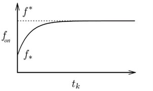
The load is secured with rigidity spring to a fixed support, Fig. 1(a). The load is acted upon by a friction force and periodic external force . The motion of the load in the direction of the motion of the belt is limited by a wall situated at distance ‘’ from the equilibrium state of the load when the belt is at halt. It is known [8] that in a mathematical model of such a kind of system, not accounting for the external force, the wall or the heredity of the dry friction force, there exists only one stable limiting cycle in its phase space. It is assumed in the present work that sliding friction coefficient is a constant value, whereas the state friction coefficient, according to the hypothesis of А. Yu. Ishlinskiy and I. V. Kragelskiy [1], is a continuous non-decreasing function of time of a prolonged contact (identity of the velocities of the load and the belt) of these bodies Fig. 1(b). In the present work, Coulomb-Hammonton friction is taken as a mathematical model of sliding friction forces. The impact against the wall is assumed to be instantaneous, with restoring coefficient .
The mathematical model of the system in question can be written as:
where the first equation describes the law of the motion of the body, taking account of sliding friction coefficient , with a velocity differing from the velocity of the belt; the second inequality postulates the ratio of forces providing the motion of the belt at a velocity equal to the velocity of the belt, accounting for the form of the coefficient of friction of relative rest (CFRR) – (Fig. 1(b)). The third equation describes the model of an impact of the load against the wall.
Introducing dimensionless time variable and parameter , system Eqs. (1)-(3) can be rewritten as:
where and is dimensionless external force.
1.2. The phase space structure
As the system is non-autonomous and described by a second-order differential equation of a variable structure, its state is triplet and the phase space is, accordingly, three-dimensional. Any trajectories in it can exist only within half-space . The phase space is divided by plane into subspaces and , in which the behavior of phase trajectories is described by the following equations, respectively:
It can be shown that in plane there exist a plate of sliding motions [8-9] , limited by curves and :
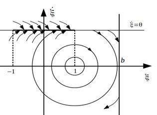
Fig. 2 depicts a projection of a phase space onto plane for a zero external force.
Fig. 2A projection of a phase space
1.3. Dynamics of the system
In what follows, it is assumed that , and dimensionless functional relation of CFRR , where is time of prolonged contact, is a piecewise-continuous function of the form:
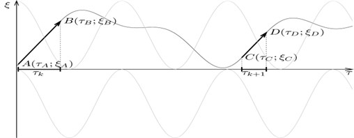
As the mapping point almost invariably gets onto the sliding motion plate, the dynamics of the system can be analyzed by studying either the properties of the point mapping of boundary onto itself, or the properties of a numerical sequence, with its elements being equal to times , . Motions with prolonged stops (MPS) along plane are shown in Fig. 3 with arrows.
Fig. 3A portrait of phase trajectories with prolonged stops
Let , be a sequence of points along surface , not belonging to the sliding motion plate and defined by Eq. (10) for , and Eq. (11) for , the coordinates of initial point being , , . Then one can find such n that point following will invariably belong to sliding motion plate , and its motion will be defined by Eq. (9) as long as relation , , ; , , holds. Let be a point transform of points , and a transform of points , . It is evident that mapping point will get onto the sliding motion plate after n transforms of the form , , Then the equations relating two successive times , of the motion of the mapping point along the sliding motion plate up to the ‘floating boundary’ can be written as:
where are determined from the solutions of the following system of equations:
Introducing into consideration functions:
One can write the following relation between the two successive times , of the combined motion of the body and the belt (MPS):
where is number of points .
To analyze the dynamics of the system in question using Poincare function, a software product has been developed on a Java platform, which makes it possible to compute, for various parameters of the system, phase trajectories, type of Poincare functions and bifurcation diagrams.
1.4. Results of numerical experiments
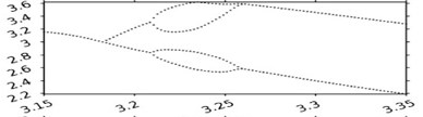
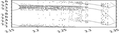
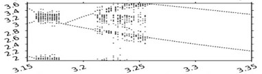
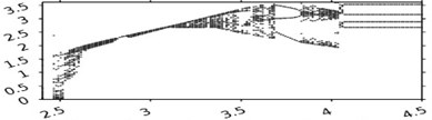
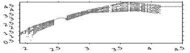
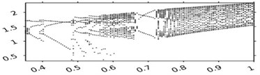
Fig .4 shows bifurcation diagrams demonstrating the dynamic effect of the wall on the behavior of the system. The horizontal axis corresponds to the variable parameter, the vertical one shows the duration of the combined motion of the body with the belt. In Fig. 4, the velocity of the belt was assumed to depend on the time according to the cosinusoidal law. A variable parameter in these diagrams is frequency of the time-dependence of the velocity of the belt. Fig. 4(a) depicts a bifurcation diagram of the system without a wall. In constructing the diagram, the external force was taken to be equal to zero, the velocity of the belt to be described by function , and parameter of piecewise-linear function of CFRR to be equal to 3. Figs. 4(b) and Fig. 4(c) differ from Fig. 4(a) only in the presence of a wall. In both diagrams, the value of the velocity recovery coefficient during the impact is chosen to be 0.5, whereas the coordinate of the wall is 4.025 and 4.05, respectively. Fig. 4(d) shows the effect of changing the coordinate of the wall on one of the cross-sections of Fig. 4(a). In Fig. 4(d), all the parameters coincide with those chosen for Fig. 4(a), the value of being equal to 3.22. Figs. 4(e) and Fig. 4(f) present diagrams on the coordinate of the wall and the velocity recovery coefficient during the impact for the same parameter values, respectively. The velocity of the belt was chosen to be 1. The external force function is expressed as , parameter of piecewise-linear function of CFRR is equal to 3, the wall coordinate 2, coefficient 0.5.
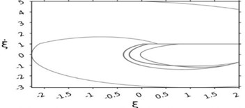
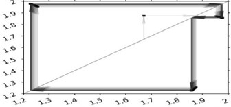
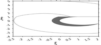
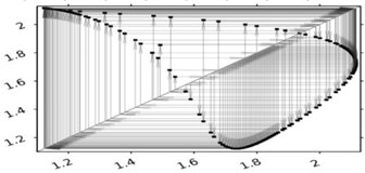
Fig. 5 depicts phase portraits and Lamerey diagrams for two sets of parameter values corresponding to two cross-sections of Fig. 4(f). Lamerey diagrams are constructed based on the durations of combined motion of the body and the belt. Figs. 5(a) and 5(b) correspond to the following parameter values: parameter (SFRR) is equal to 3, velocity of the belt is equal to 1, the external force is variable , wall coordinate is 2, coefficient 0.7. Figs. 5(c) and 5(d) differ only in the value of coefficient 0.75. It is evident from Fig. 5 that for the value of coefficient 0.7 the system has a stable limiting cycle with three stops of the form OHBOHBOHB, i.е., the first stop “O” is followed by an impact against the wall “H” and then by portion “B” in half-space , which is followed by two more similar turns of OHB, and then the cycle is repeated. For 0.75, the behavior of the system is chaotic.
Fig. 4Bifurcation diagrams for various values of parameter b – the position of the vibration limiter
a)
b)
c)
d)
e)
f)
Fig. 5Phase portraits and the chart Lameria
a)
b)
c)
d)
2. Conclusions
The dynamics of a non-autonomous shock-vibrating system consisting of a pair of bodies of friction has been studied using a numerical-analytical approach, implementing the mathematical apparatus of the point mapping method, accounting for hereditary-type dry friction forces in the presence of a vibration limiter. The specificity of the approach is in that a point mapping is formed not classically (mapping Poincare surface onto itself), but based on the duration of the relative rest of the load and the belt, which considerably simplified the process of point mapping and its detailed analysis.
Based on the character of changes in the bifurcation diagrams, the authors have determined the main laws of changes in the motion regimes (occurrence of random complexity periodic motion regimes and possible transfer to chaos via the period doubling process) when changing the parameters of the vibration system.
References
-
Ishlinskiyi A. Yi., Kragelskiyi I. V. About racing in friction. Journal of Technical Physics, Vols. 4-5, Issue 14, 1944, p. 276-282.
-
Kahenevskiyi L. Ia. Stochastic auto-oscillations with dry friction. Inzh-fiz Journal, Vol. 47, Issue 1, 1984, p. 143-147.
-
Vetukov M. M., Dobroslavskiyi S. V., Nagaev R. F. Self-oscillations in a system with dry friction characteristic of hereditary type. Journal Proceedings of the USSR Academy of Solid Mechanics, Vol. 1, 1990, p. 23-28.
-
Metrikin V. S., Nagaev R. F., Stepanova V. V. Periodic and stochastic self-oscillations in a system with dry friction hereditary type. Journal Applied Mathematics and Mechanics, Vol. 5, Issue 60, 1996, p. 859-864.
-
Leine R.I., van Campen D.H., De Kraker A. Stick-slip vibrations induced by alternate friction models. Journal Nonlinear Dynamics, Vol. 16, 1998, p. 41-54.
-
Leine R.I., van Campen D.H., De Kraker A. An approximate analysis of dry friction-induced stick-slip vibrations by a smoothing procedure. Journal Nonlinear Dynamics, Vol. 19, 1999, p. 157-169.
-
Leine R.I., van Campen D.H. Discontinuous fold bifurcations in mechanical systems. Archive of Applied Mechanics, Vol. 72, 2002, p. 138-146.
-
Feygin M. I. Forced Oscillations of Systems with Discontinuous Nonlinearities. Science, 1994, p. 285.
-
Neymark Yu. I. The Method of Point Mappings in the Theory of Nonlinear Oscillations. Science, 1972, p. 471.
-
Shuster G. Deterministic Chaos. Peace, 1988, p. 237.
About this article

The research was supported by the Russian Science Foundation, Grant No.16-19-10237.
