Abstract
The method based on a particle filter for a fatigue crack growth prognosis has proved to be a powerful and effective tool for developing prognostics and health management (PHM) technology. However, the widely used basic particle filter have the unavoidable particle impoverishment problem, which will make particles unable to approximate the true posterior probability density function of the system state and lead to a prognosis result with a large error. This paper proposes a fatigue crack growth prognosis method based on a deterministic resampling particle filter. The active structural health monitoring based on the Lamb wave is used for on-line crack length monitoring with piezoelectric transducers. With the on-line crack measurement, the crack state and crack growth model parameters are estimated for a fatigue crack growth prognosis. In addition, the deterministic resampling procedure is employed to overcome the particle impoverishment problem. The result shows the proposed crack growth prognosis method based on deterministic resampling particle filter can provide more satisfactory results than the basic particle filter.
1. Introduction
Prognostics and health management (PHM) technology [1, 2], which obtains actual conditions via advanced sensors and system remaining the useful life through prognostic methods, is an immediate area of research focus for safety-critical engineer systems such as aircrafts, power plants and infrastructures. By adopting PHM technology, scheduled maintenance can be replaced by condition-based maintenance with safety improvement and cost reduction.
Fatigue crack is regarded as a primary degradation process affecting the structural integrity. The prognosis of fatigue crack growth is a crucial problem for developing the PHM technology. Traditional crack growth models are accurate if model parameters have been accurately defined [3]. However, fatigue crack growth is a stochastic process affected by numerous uncertainties, which arise from sources such as intrinsic material properties, loading, and environmental factors. Crack would grow in different ways even in identical components working under the same condition. To deal with these uncertainties, studies are carried out to integrate actual crack measurements obtained from sensors with crack growth models using the Bayesian theory, which come out to be the estimation problem of the crack state and crack growth model parameters using a sequence of noise measurements. For the estimation problem of a dynamic system, the Kalman filter (KF) offers the optimal solution for linear systems affected by Gaussian noise [4]. However, the fatigue crack growth process is nonlinear and affected by non-Gaussian noise. Further, modified KFs such as the extended KF and the unscented KF are developed to extend the KF to the nonlinear system. But they still need the Gaussian noise assumption, and poor performance will be obtained when the system is highly nonlinear [5]. On the other hand, the particle filter (PF) is capable of handling nonlinear and/or non-Gaussian systems without restrictive assumptions, which core idea is to approximate the posterior probability density function (PDF) of the system state by a set of random samples called as particles with associated weights. Recently, the PF is more and more applied for predicting problems [6-9], especially for the fatigue crack growth prognosis [10-18].
However most studied cases mentioned above adopt the basic PF algorithm also known as the sequential importance sampling and resampling (SIR) [19], which has the inherent problem called as the particle impoverishment. Due to the multinomial resampling algorithm [20] adopted in the SIR algorithm, particles are duplicated and eliminated only depending on the corresponding particle weights. Particles that have large weights are statistically selected many times, so that most particles will be replications of the same particle after several iterations and are unable to approximate the true posterior PDF. This problem leads to a large error in the prognosis of fatigue crack growth, especially when a small number of particles is required for on-line application. Cadini et al. [11], Zio et al. [12], Neerukatti et al. [13] and Chen et al. [14] developed the fatigue crack growth prognosis method based on the basic PF method, but did not discuss the particle impoverishment problem.
Several ways were proposed in the PF theory to deal with the particle impoverishment problem. The roughening [4] or the kernel smoothing [21] procedure added a random jitter to each particle after resampling to rejuvenate the particle diversity. This kind of ways is simple. For the fatigue crack growth prognosis, Orchard et al. [10], Chiachío et al. [17], and Sbarufatti et al. [18] adopted the roughening procedure in the basic PF based crack growth prognosis method, an artificial noise is added to the particle after resampling to rejuvenate the particle diversity. However, the parameters (e.g., the variance of the artificial noise or the kernel bandwidth) are customized to specific problems and need to be carefully chosen. In addition, only in specific classes of model, it is possible to draw particles directly from the analytical kernel PDF. Besides, the methods such as the auxiliary variable method [22], the Markov Chain Monte Carlo method [23] and artificial intelligent methods [24] are adopted to move particles to positions with a high likelihood region to fight the particle impoverishment problem. Corbetta et al. [15] integrated the Markov chain Monte Carlo (MCMC) sampling into the basic crack growth prognosis method based on the PF, new particles are sampled by using the MCMC sampling at each iteration, and thus the particle diversity is kept. However, the MCMC sampling procedure is computationally expensive. all these methods mentioned above are focused on the likelihood weight and ignore the spatial distribution of particles. The impoverishment problem will be serious when the sample size is small. Put differently, Li et al. [25] developed a novel deterministic resampling procedure to solve the particle impoverishment problem, which considers both the weights of particles and their spatial distribution. It is proved that the deterministic resampling can be strictly unbiased and maintains the original state density distribution. Moreover, it is quite useful when a small number of particles are required for the on-line application.
To improve the accuracy of the PF based on-line fatigue crack growth prognosis, this paper applies the deterministic resampling particle filter (DRPF) to the fatigue crack growth prognosis. The PF state vector consists of the crack length and the crack growth model parameters. Each time a new on-line crack measurement is available, it is input into the DRPF to calculate the particle weight. Based on the posterior PDF, the crack growth prognosis procedure is conducted. To overcome the particle impoverishment problem, deterministic resampling is performed so that new particles are generated from copy particles and support particles according to the weights of particles and their spatial distribution. Finally, the proposed method is validated with the fatigue test of edge crack specimens. During the fatigue test, the active structural health monitoring (SHM) based on the Lamb wave [14] is employed for on-line crack monitoring. The damage index extracted from the Lamb wave signals is used as the measurement of the crack length.
The rest of the paper is organized as follows. In Section 2, the DRPF based fatigue crack growth prognosis method is introduced. In Section 3, the fatigue test of edge crack specimens is presented, and the proposed method is validated with this fatigue test data. Finally, the conclusion is provided in Section 4.
2. Fatigue crack growth prognosis based on deterministic resampling particle filter
2.1. Fatigue crack growth prognosis based on particle filter
In the PF theory, a state space model, which consists of a state equation and a measurement equation, needs to be defined. The state equation describes the state evolution representing a hidden Markov process of order one, as shown in Eq. (1). The measurement equation governs the relationship between the measurement value and the system state, as shown in Eq. (2):
where is the discrete time index, is the system state, is a nonlinear model representing the state evolution from time to time , is the model parameter vector, is a random variable representing the state noise; is the state measurement of the state , represents the relationship between the measurement and the state , is a random variable denoting representing the measurement noise.
For solving fatigue crack growth problem, the state equation can be determined by a physic-based crack growth model. The Paris’ law [26] has been widely used, giving the crack growth rate as Eq. (3):
where is the crack length, is the number of loading cycles, and are the material constants, is the stress intensity factor (SIF) range acting as the crack growth force, which is expressed as Eq. (4):
where is the stress amplitude, is the geometric coeffecient.
Eq. (3) can be expressed in a discrete form to represent the crack evolution from time to time as expressed in Eq. (5):
where is the discrete step of loading cycles, the product gives the crack length increment for each time step. The random variable follows the Gaussian distribution , , and the term that is nonnegative is incorporated for representing uncertainties during the fatigue crack growth [27]. Thus, is lognormally distributed. The mean value of is selected as such that the expectation of is equal to 1 [15].
To express the uncertainty between different structures, the parameter is considered as a random variable and the material parameter is adopted as a constant. Thus, the PF state vector is represented as . As a result, the state equation is expressed as Eq. (6):
On the other aspect, the measurement function is defined to express the relationship between the measurement and the crack length. By using the SHM technologies, the crack length can be monitored on-line. Among SHM methods, the active guided wave based method is one of the most appealing and effective methods, which have the advantages including the sensitivity to a small damage as well as the ability of region monitoring [28, 29]. The quantity extracted from guided wave signals called as the damage index is usually applied to quantify the crack length. Thus, the measurement equation can be denoted as Eq. (7):
where the random variable follows the Gaussian distribution (, ), denoting that the damage index is affected by zero mean Gaussian noise, is a one-to-one mapping between the crack length and the damage index dominated by models such as polynomial or artificial neural network.
At the current time , the PF objective is to calculate the posterior PDF of the system state, conditioned on the measurements {, , ..., }. This posterior PDF can be evaluated with the well-known iterative prediction and updating steps according to the Chapman-Kolmogorov equation and the Bayes’ rule [30]. However, this iterative procedure does not have analytical solutions in most cases. The PF deals with it by using the Monte Carlo method: the posterior PDF is approximated by a set of random samples , 1, ..., called as “particles” with associated weights , 1, ..., , shown in Eq. (8):
where is the number of particles and is sampled from a PDF called as the importance density. is the Dirac delta function. In the basic PF, the weight is calculated through the likelihood value of each particle, as shown in Eq. (9):
As the measurement equation defined in Eq. (7), the particle weight updating is performed as Eq. (10):
After that, the weight normalization as Eq. (11) is performed to ensure the sum of weights being equal to 1:
As a result, the posterior estimation of the system estimate can be evaluated as the weighted summation of the particles:
Based on the posterior PDF of the state , a prognosis of the future state evolution is performed by projecting the particles in the posterior PDF in time up to the future as follows:
where is the future time of interest.
2.2. Deterministic resampling
In Eq. (11), the variance of particle weights can only increase overtime [30], so that the particle weight will concentrate on a few particles and most particles will have negligible weights. The basic particle filter adopts the multinomial resampling algorithm, which draws a new particle set from , 1, ..., with the probability proportional to the normalized weight , 1, ..., . If the weight of the th particle is large, this particle is duplicated as several particles, otherwise this particle will not be contained in the new particle set. The size of the new particle set keeps being equal to , and the total particle weight is set to . However, this procedure brings the side effect of sample impoverishment problem that most particles are replications of the same particle after several iterations. To overcome the sample impoverishment problem, the deterministic resampling particle filter [25] is adopted in this paper, where the deterministic resampling procedure is conducted after the weight normalization.
The deterministic resampling procedure generates particles from two parts: (1) copy particles; (2) support particles.
1) Copy particles:
For the th particle , it is duplicated for times, where is the integer part of the product , as shown in Eq. (15):
where the symbol means the integer part. For all particles, total copy particles are obtained, what is denoted as .
After that, the residual weight of each particle is evaluated as Eq. (16):
2) Support particles:
Instead of uncensored discarding particles that have small weights, the state space of particles is partitioned into variable-size countable units considering the residual weight of the particle and their spatial distribution. Assuming the particle set with residue weights is divided into spatial grids. The th grid is denoted as Eq. (17):
where the subscript denotes the index of partition grid 1, 2,…, , is the number of particles contained in the th grid and is defined as the particle density. If a grid is without any particles, it is called an empty grid.
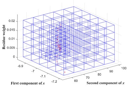
The partition of the spatial distribution is initialized with a starting grid size , which does not have more dimensions than the state space. All particles are first partitioned into grids of size . Then the particle density of each nonempty grid is detected: if it is more than a predefined threshold , the grid is subdivided into half size in all dimensions; otherwise, the grid is considered as an independent one. This detection and partition procedure is repeated until the particle density of all grids is below or the grid size is lower than the threshold bound . Here, is a pre-set threshold, which prevents grids from being divided into portions of too small size [25]. Fig. 1 shows a partition when the state has two dimensions. Particles are located in several grids according to their state values and residue weights.
Fig. 1Illustration of spatial grids of deterministic resampling
After the spatial partition is completed, particles are sampled from these grids, called as support particles. Assuming the total non-empty grids are obtained, a support particle is obtained for the th nonempty grid, 1, 2, 3, ..., , as shown in Eq. (18):
where symbol denotes the summing up. The weighted summation of the particles in the partition grid is deemed as the newly resampled particle . The summation of the particle weights in this partition grid is adopted as a new weight of the resampled particle. Through this procedure, the deterministic resampling preserves low-weight particles during resampling for possible usages in the future [25].
The weight of the copy particle , 1, 2, 3, ..., , is specified as the equal division of the complement of the support particle weights, as expressed in Eq. (19):
The resampled particle set consists of the copy particles and support particles . It should be noted that the particle number changes along with the iteration, which is no longer a fixed number.
2.3. Implementation of proposed fatigue crack growth prognosis method
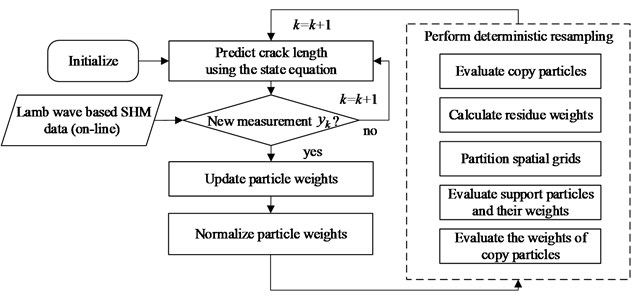
Fig. 2 shows the framework of the proposed fatigue crack growth method. While the structure is under service and monitored with the active Lamb wave based SHM, the measurement of the crack length is sequentially obtained and inputted into the DRPF. Once a new measurement is available, it is used to update particle weights. Thus, the posterior PDF is calculated and is the basis of the crack growth prognosis. After that, deterministic resampling is conducted to resample particles from the spatial distribution of particles, and the newly obtained particles are transferred to the next time step.
Fig. 2Framework of fatigue crack growth prognosis based on DRPF
3. Experimental evaluation on edge crack specimens
3.1. Experimental setup
Five edge-crack specimens are manufactured using a LY12 aluminum plate of 2 mm thickness, as illustrated in Fig. 3, which geometry and sensor layout are shown in Fig. 4. These specimens are labeled as T1, T2, T3, T4 and T5. A notch of length is machined at the specimen edge to initiate the crack and control the direction of crack growth. The notch length is selected as 50 mm to accelerate the fatigue tests. Two columns of holes at each end of the specimen are used to assemble the fixture with bolts.
Fig. 3Edge crack specimen
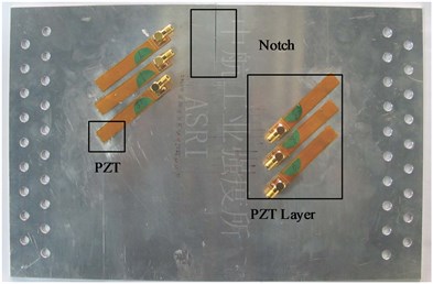
Fig. 4Geometry and PZT layout
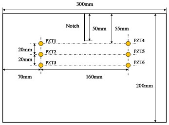
During the fatigue test, the active Lamb wave based SHM is employed to monitor the crack growth in real time. Encapsulated piezoelectric transducers called as peizoelectric transducer (PZT) layers [31] are adhered to the surface of specimen for exciting and acquiring guided wave signals. Totally six PZTs are attached on the surface of each specimen. These PZTs are numbered as PZT1, PZT2, PZT3, PZT4, PZT5, PZT6 respectively, where PZT1, PZT2, PZT3 are used as the actuators, and the others are employed as the sensors. The signal transmitting path, where the signal is excited with PZT1 and sensed with PZT4, is denoted as Channel 1-4. Totally three Channels are employed: Channel 1-4, Channel 2-5, and Channel 3-6, which have different distances from the crack tip.
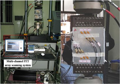
Fig. 5 illustrates the experimental setup of the fatigue test. The MTS electro-hydraulic servo material test system is used for applying the fatigue load. The specimen is clamped with the fixture at the both ends. The multi-channel PZT array scanning system developed by the authors’ group [32] is adopted for signal actuating and acquiring. Before fatigue tests, a tensile test is performed with T1 specimen to determine the fracture load of the cracked specimen. As a result, the fracture load of this specimen is 56 kN. Thus, the fatigue load of T2-T5 specimens is chosen as the sinusoid load of the peak value 17 kN, stress ratio 0.1 and 10 Hz load frequency. The experimental crack length is observed at 5mm interval, while the Lamb wave based crack monitoring is performed. The 5-cycle Hanning-windowed sine burst signal with the center frequency of 250 kHz and ±70 V amplitude is used as the excitation signal, and the response Lamb wave signals are acquired from three channels with the 10 MHz sample rate.
Fig. 5Experimental setup
3.2. Experimental results
Fig. 6 shows the fatigue crack growth trajectories of T2-T5 specimens observed at 5 mm interval. It can be found, although the specimen and fatigue loads are identical, these fatigue crack growth trajectories are diverse. This is because the fatigue crack growth process is a stochastic process, which is affected by numerous uncertainties derived from sources such as the intrinsic material property, specimen machining and assembling error [27]. Thus, crack growth prognosis made by a deterministic physical model may cause a large error.
Fig. 6Experimental crack lengths versus loading cycles of T2-T5 specimens
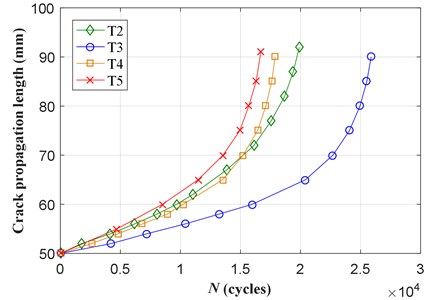
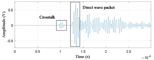
Fig. 7 illustrates a typical Lamb wave signal acquired from the Channel 2-5 with PZTs. The crosstalk is caused by the excitation signal which is a 5-cycle Hanning-windowed sine burst. The direct wave packet is the first wave packet transmitted from the actuator to the sensor, thus it carries the most important information of the crack growth process. The amplitude and phase of the direct wave packet changes with the increase of the crack length. These changes can be used to represent the crack growth. A quantity called as the damage index is usually employed to quantify the changes between changed signals and the signal collected at the pristine state called as the baseline signal. The normalization correlation moment (NCM) damage index [33] is adopted in this paper, which is expressed as Eq. (20):
where is the damage index, is the cross-correlation function of the baseline signal that is collected at the pristine state and the signal collected during the crack growth, is the autocorrelation function of the signal , is the signal length, is the order of the statistical moment that is arbitrary and not limited to integers.
Fig. 7Typical lamb wave signal acquired from channel 2-5
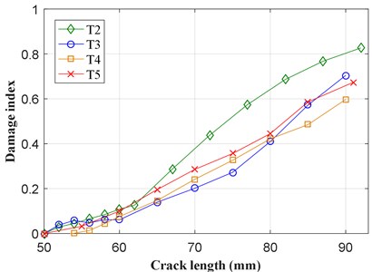
To calculate the NCM damage index, the direct wave packet is used instead of the whole signal. The baseline signal is collected when each specimen is clamped, and the crack does not start to grow. As shown in Fig. 4, there are three channels, the damage index calculated is different from other channels because the positions of these channels are different from each other. After comparison, damage indices extracted from Channel 2-5 represent good correlation with crack lengths of T2-T5 specimens, as shown in Fig. 8, which are calculated with the statistical moment 1.
Fig. 8Experimental crack length versus NCM damage index
3.3. Validation of the proposed DRPF based on-line fatigue crack growth prognosis
To validate the method, the last T5 specimen is used as the target structure to validate the proposed method. Thus, the fatigue test data of T2-T4 specimens are employed as the database to establish the state space model of edge-crack specimen.
3.3.1. State space model of edge-crack specimen
In the state equation defined for fatigue crack growth, as shown in Eq. (5), the SIF range of the edge-crack plate can be calculated through Eq. (21) referring to the SIF handbook [34]:
where is the nominal stress amplitude, is the length of the edge crack, is the width of the edge-crack plate, is the geometric correction factor which is the function of the ratio . This correction factor is expressed as follows:
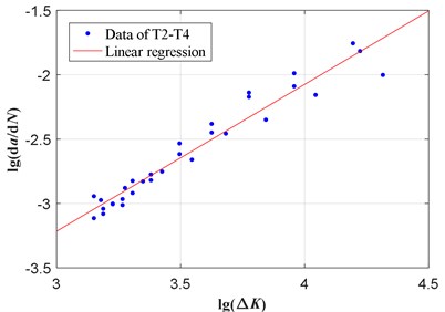
Usually, the parameters and in the Paris’ law is obtained with fatigue test data of the same specimens. In this paper, the crack growth data of T2-T4 specimens is used to fit these parameters to describe the prior knowledge of fatigue crack growth of edge crack specimen. The logarithm transformation of the Paris’ law gives Eq. (23):
where and are the intercept and slope of the linear relationship between and the crack growth rate . The data points of the crack growth rate can be approximated by applying the commonly used secant method [35]. Fig. 9 illustrates the data points of T2-T4 specimens. Through linear regression, the fitted parameters are obtained as 3.819 and –13.624.
To express the uncertainty between different structures, the parameter is considered as a random variable, and the material parameter in Eq. (6) is adopted as a constant. The uncertainty of the material parameter is considered in the crack growth model. The prior distribution of the parameter is adopted as (–13.624, 0.32), in which 0.32 is adopted so that it is efficient to represent the dispersion of the crack growth regulated by the Paris’ law.
Fig. 9Linear regression for Paris model parameters
In the measurement equation, shown in Eq. (17), the measurement mapping represents the relationship between the crack length and the measured crack length. With the experimental results of T2-T4 specimens shown in Fig. 8, this mapping can be obtained by polynomial fitting as Eq. (24):
where is the crack length, 50 mm is the initial crack length (notch length).
Thus, the measurement equation is expressed as follows:
where denotes the measurement uncertainty. The variance 0.064 is also calculated with the experimental results of T2-T4 specimens by using the maximum likelihood estimation.
3.3.2. Fatigue crack growth prognosis of T5 specimen
T5 specimen is used as the target structure to validate the proposed DRPF based crack growth prognosis method. For the on-line crack growth prognosis of T5 specimen, the DRPF parameter is set as 50, 50, and 0.01. The starting grid size [, , ] of the state space partition in deterministic resampling is adopted as:
At the initial time 0, random samples are drawn from the distribution (–13.624, 0.32) and assigned to each particle and the particle set is initialized as 1,...,. Meanwhile, the weight of each particle is initialized as , 1,..., .
During the fatigue test of T5 specimen, guided wave signals are excited and acquired sequentially. The damage index is extracted from these signals as the measurement of the actual crack length, which is employed to calculate the particle weight. Thus, the posterior PDF of the crack length and parameter is obtained as the approximation with the help of the particles , 1, ..., and associated weights . Based on the posterior PDF, crack growth prognosis is performed. And then the deterministic resampling is conducted according to the spatial distribution of the particles. As mentioned above, the particles are initialized with . After each resampling procedure, values in are duplicated and eliminated for each particle. Thus, the particle diversity can be represented by counting the unique values of particles. Fig. 10 illustrates the varying number of different particles after resampling processes when new measurements are available. It can be found that the particle impoverishment problem of the basic PF is serious only after several resampling procedures. By contrast, the DRPF maintains a diversity particle set.
Fig. 10Varying number of unique C values after resampling processes
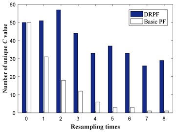
Fig. 11Posterior estimate of the crack length considering all the crack measurements
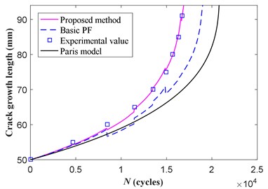
During on-line prognosis, the posterior PDF of the crack length and parameter is used as the initial conditions for prognostic routines. Fig. 11 illustrates the prognosis results given by the basic PF and DRPF. In this figure, the crack growth trajectory of the Paris model represents the result by using the Paris’ law with the fitted parameter –13.624, 3.819, and 50, 50, which results in the biggest error. The prognosis result of the basic PF slightly improved by considering the actual crack measurement, however there is still a large error because of particle impoverishment. On the other hand, the DRPF gives quite a good result. The root means square error (RMSE) of the basic PF and DRPF is 1.5 mm and 10.5 mm respectively, showing the effectiveness of the proposed method.
4. Conclusions
To improve the prognosis accuracy, the deterministic resampling particle filter is applied to the fatigue crack growth prognosis. In the DRPF based method, the crack length and the parameter in the crack growth model are estimated simultaneously. The deterministic resampling procedure draws particles from two sources: copy particles and the support particles, which maintain the particle diversity and overcome the particle impoverishment problem. A fatigue test of edge-crack specimens is conducted to validate the proposed DPRF based fatigue crack growth method, during which the active structural health monitoring based on the Lamb wave is performed to offer the on-line crack measurement. The validated result shows better performance of the proposed method than the basic PF. Although the effectiveness of the proposed method has been proved, further detail research still needs to be performed on more realistic and complex structures.
References
-
Tsui K. L.,Chen N., Zhou Q., Hai Y., Wang W. Prognostics and health management: A review on data driven approaches. Mathematical Problems in Engineering, Vol. 6, 2015, p. 1-17.
-
Lee J., Wu F., Zhao W., Ghaffaria M., Liao L., Siegel D. Prognostics and health management design for rotary machinery systems – Reviews, methodology and applications. Mechanical Systems and Signal Processing, Vol. 42, Issue 1, 2014, p. 314-334.
-
Huang M., He J., Guan X. Probabilistic inference of fatigue damage growth with limited and partial information. Chinese Journal of Aeronautics, Vol. 28, Issue 4, 2015, p. 1055-1065.
-
Arulampalam M. S., Maskell S., Gordon N., Clapp T. A tutorial on particle filters for online nonlinear/non-Gaussian Bayesian tracking. IEEE Transactions on Signal Processing, Vol. 50, Issue 2, 2002, p. 174-188.
-
Yin S., Zhu X. Intelligent particle filter and its application to fault detection of nonlinear system. IEEE Transactions on Industrial Electronics, Vol. 62, Issue 6, 2015, p. 3852-3861.
-
Talha M., Stolkin R. Particle filter tracking of camouflaged targets by adaptive fusion of thermal and visible spectra camera data. IEEE Sensors Journal, Vol. 14, Issue 1, 2014, p. 159-166.
-
Jouin M., Gouriveau R., Hissel D., Péra M. C., Zerhouni N. Particle filter-based prognostics: Review, discussion and perspectives. Mechanical Systems and Signal Processing, Vol. 72, 2016, p. 2-31.
-
Fan J., Yung K. C., Pecht M. Predicting long-term lumen maintenance life of LED light sources using a particle filter-based prognostic approach. Expert Systems with Applications, Vol. 42, Issue 5, 2015, p. 2411-2420.
-
Samadi M. F., Alavi S. M. M., Saif M. An electrochemical model-based particle filter approach for Lithium-ion battery estimation. 51st IEEE Conference on Decision and Control, 2012, p. 3074-3079.
-
Orchard M. E., Vachtsevanos G. J. A particle-filtering approach for on-line fault diagnosis and failure prognosis. Transactions of the Institute of Measurement and Control, Vol. 31, Issues 3-4, 2009, p. 221-246.
-
Cadini F., Zio E., Avram D. Model-based Monte Carlo state estimation for condition-based component replacement. Reliability Engineering and System Safety, Vol. 94, Issue 3, 2009, p. 752-758.
-
Zio E., Peloni G. Particle filtering prognostic estimation of the remaining useful life of nonlinear components. Reliability Engineering and System Safety, Vol. 96, Issue 3, 2011, p. 403-409.
-
Neerukatti R. K., Hensberry K., Kovvali N., Chattopadhyay A. A novel probabilistic approach for damage localization and prognosis including temperature compensation. Journal of Intelligent Material Systems and Structures, Vol. 27, Issue 5, 2016, p. 592-607.
-
Chen J., Yuan S., Qiu L., Cai J., Yang W. Research on a lamb wave and particle filter-based on-line crack propagation prognosis method. Sensors, Vol. 16, Issue 3, 2016, p. 320.
-
Corbetta M., Sbarufatti C., Manes A., Giglio M., Corbetta M., Sbarufatti C. On dynamic state-space models for fatigue-induced structural degradation. International Journal of Fatigue, Vol. 61, Issue 4, 2014, p. 202-219.
-
Orchard M. E., Vachtsevanos G. J. A particle filtering approach for on-line failure prognosis in a planetary carrier plate. International Journal of Fuzzy Logic and Intelligent Systems, Vol. 7, Issue 4, 2007, p. 221-227.
-
Chiachío J., Chiachío M., Sankararaman S., Saxena A., Goebel K. Condition-based prediction of time-dependent reliability in composites. Reliability Engineering and System Safety, Vol. 142, 2015, p. 134-147.
-
Sbarufatti C., Corbetta M., Manes A., Giglio M. Sequential Monte-Carlo sampling based on a committee of artificial neural networks for posterior state estimation and residual lifetime prediction. International Journal of Fatigue, Vol. 83, 2016, p. 10-23.
-
Gordon N. J., Salmond D. J., Smith A. F. M. Novel approach to nonlinear/non-Gaussian Bayesian state estimation. IEE Proceedings F-Radar and Signal Processing, Vol. 140, Issue 2, 1993, p. 107-113.
-
Hol J. D., Schon T. B., Gustafsson F. On resampling algorithms for particle filters. Nonlinear Statistical Signal Processing Workshop, 2006, p. 79-82.
-
Musso C., Oudjane N., Legland F. Improving regularized particle filters. Sequential Monte Carlo Methods in Practice, Springer-Verlag, New York, 2001, p. 247-272.
-
Pitt M. K., Shephard N. Filtering via simulation: Auxiliary particle filters. Journal of the American statistical association, Vol. 94, Issue 446, 1999, p. 590-599.
-
Andrieu C., Doucet A., Holenstein R. Particle Markov chain Monte Carlo methods. Journal of the Royal Statistical Society: Series B (Statistical Methodology), Vol. 72, Issue 3, 2010, p. 269-342.
-
Li T., Sun S., Sattar T. P., Corchado J. M. Fight sample degeneracy and impoverishment in particle filters: a review of intelligent approaches. Expert Systems with Applications, Vol. 41, Issue 8, 2014, p. 3944-3954.
-
Li T., Sattar T. P., Sun S. Deterministic resampling: unbiased sampling to avoid sample impoverishment in particle filters. Signal Processing, Vol. 92, Issue 7, 2012, p. 1637-1645.
-
Paris P. C., Erdogan F. A critical analysis of crack propagation laws. Journal of Basic Engineering. Vol. 85, Issue 4, 1963, p. 528-533.
-
Yang J. N., Manning S. D. Stochastic crack growth analysis methodologies for metallic structures. Engineering Fracture Mechanics, Vol. 37, Issue 5, 1990, p. 1105-1124.
-
Su Z., Ye L. Identification of Damage Using Lamb Waves: from Fundamentals to Applications. Springer Science and Business Media, New York, 2009.
-
Giurgiutiu V. Structural Health Monitoring: with Piezoelectric Wafer Active Sensors. Academic Press, Manhattan, 2007.
-
Doucet A., Godsill S., Andrieu C. On sequential Monte Carlo sampling methods for Bayesian filtering. Statistics and Computing, Vol. 10, Issue 3, 2000, p. 197-208.
-
Qiu L., Yuan S., Shi X., Huang T. Design of piezoelectric transducer layer with electromagnetic shielding and high connection reliability. Smart Materials and Structures, Vol. 21, 7, p. 2012-75032.
-
Qiu L., Yuan S. On development of a multi-channel PZT array scanning system and its evaluating application on UAV wing box. Sensors and Actuators A: Physical, Vol. 151, Issue 2, 2009, p. 220-230.
-
Torkamani S., Roy S., Barkey M. E., Sazonov E., Burkett S., Kotru S. A novel damage index for damage identification using guided waves with application in laminated composites. Smart Materials and Structures, Vol. 23, Issue 9, 2014, p. 095015.
-
Tada H., Pars P, C., Irwin G. R. The Stress Analysis of Cracks. Handbook, Del Research Corporation, 1973.
-
ASTM International Standard Test Method for Measurement of Fatigue Crack Growth Rates. ASTM, 2011.
Cited by
About this article

This work is supported by Key Program of National Natural Science Foundation of China, Grant No. 51635008, National Natural Science Foundation of China, Grant No. 51575263, Qing Lan Project of Jiangsu Province of China, the Priority Academic Program Development of Jiangsu Higher Education Institutions of China, Funding of Jiangsu Innovation Program for Graduate Education, the Fundamental Research Funds for the Central Universities.
