Abstract
Human body experiences a long natural evolution to have good movement forms and flexible driving mode, during which process, human muscles have already evolved to a sophisticated bio-actuator, usually used in the bionic design of mechanical structures. The article presents a novel idea for the bionics design of artificial limb or exoskeleton robot, considering the motion level and the driving level of human body simultaneously, i.e. the lower limb segment movement and the muscle activity. Firstly, as the support phase, the most complex process during human walking, we divided it into three sub-phases and studied each other’s variations about the angle and torque by the built motion capture system, which is important for ground reaction force control (GRF control). Secondly, the principal muscles around the knee joint were studied by biomechanical simulation, i.e. the vastus medialis muscle and the biceps femoris muscle, after the data of clinical gait by experiment was imported into the human simulation software. The result showed that the vastus medialis muscle, as Hill three elements model, was the principal muscle during knee’s extension motion, which mainly worked during the support phase and could provide a maximum force of 280 N.m. In contrast, the biceps femoris muscle, as Hill two elements model, was the principal muscle during knee’s flexion motion, which mainly worked during the swing phase and could provide a maximum force of 220 N.m.
1. Introduction
Lower limb exoskeletons have been a focus in the last decade, which are worn on the outside of human’s lower limb and able to follow the movement of human leg freely. For helping the paralyzed patients walk again or enhance the power of the wearer, the mechanism structure of the exoskeleton robots is always designed as anthropomorphic type or quasi-anthropomorphic such that the rotation axis of the robot joint aligns with the human body’s, such as HULC, XOS-2 and HAL [1, 2]. The anthropomorphic/quasi-anthropomorphic structure has excellent advantages. On the one hand the humanoid structure enables the robot cooperating with the motion of human, reducing collision between each other; on the other hand, studying the structure and gait motion of the human’s simplify the design of mechanism and control system of the human-robot cooperation system [3]. In a word, it can be seen that the method of human bionics makes the design process of exoskeleton system more economical and scientific [4, 5].
As the development of gait analysis equipment, we could analyze the kinematics and dynamics of human lower limb more precisely. The article will analyze the motion mechanism of the three lower limb joints, e.g. the hip joint, the knee joint and the ankle joint, which is significant important for exoskeleton control [6, 7]. Except for the body motion, the muscles could play an important role in helping design a perfect actuator of exoskeleton. As we know, it is the contraction of muscles that drives the movement of skeleton around the joint. So, the biomechanics of the joint muscles are studied for better understanding of human motion, which is in favor of further optimized selection of exoskeleton’s actuator and energy source.
The main research is organized as follows. Section 2 presents the experiment principle of the multi-camera motion capture system and the related experiment method. Then we will present the mathematical model of human walking and the simulation principle of relevant muscles. Section 3 analyzes the experiment results of clinic gait including kinematics and dynamics. Section 4 addresses the performance of the muscles by simulation. Section 5 concludes this paper.
2. Mathematical model of human lower limb and simulation model of relevant muscles
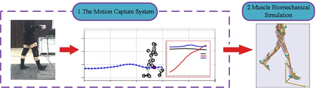
As Fig. 1 shown, to reveal the relationship between human gait and muscles, the whole process is divided into two. Firstly, the motion of human walking is obtained by the human motion capture system, after which the dynamics of each joint, i.e. the torque of the joint, is studied by the gait analysis software. Secondly, the forces of the muscles driving such human walking are calculated by inverse dynamics after the capture motion data achieved by the above experiment are inputted into the muscle biomechanical simulation software.
Fig. 1Research process
2.1. Human motion capture experiment
The experiment is divided into three steps: experiment preparation, experiment starting and experimental data analysis. Experiment preparation is to complete a series of preparations before the experiment, including setting the markers by the Helen Hayes method. Experiment starting is to enter the guidance interface, where the user could complete one time of gait motion acquisition. Experimental data analysis is to calculate the joint torque by the internal algorithm.
2.1.1. Experiment equipment
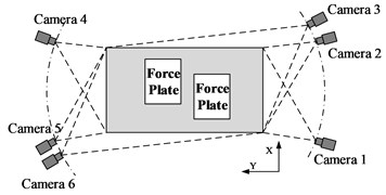
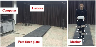
The motion capture system consists of six high speed cameras arranged in the scene, two foot force plates on the pavement (the main specifications is shown in Table. 2), a series of marked points pasted on the right positions of human body and a computer for recognizing coordinate values of marked points and calculating the dynamics of each joint, as shown in Fig. 2.
Fig. 2Human motion capture system
a)
b)
2.1.2. Set the markers
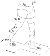
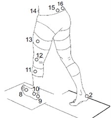
One step during the process of experiment preparation is to set the markers by rule and line. 16 markers in all were installed on the body. Markers 1-7 and markers 8-14 were attached on the left and right lower limbs separately. Marker 15 present sacral and marker 16 was used to distinguish the left and the right (as shown in Fig. 3). Take the right leg as an example, each body’s segment was constructed by three markers, as listed in Table. 3.
Table 2Main specifications
High speed camera | Foot force plates | ||
Manufactures | Point Grey Corp, Canada | Manufactures | By ourselves |
Specifications | S250e | Maximum force along X/Y/Z | 1600/1600/3200 N |
Maximum shooting speed | 250 fps | Maximum moment around X/Y/Z | 960/640/800 Nm |
Dpi | 832 (H)×832 (V) | Number | 2 pieces |
Number | 6 pieces | Sensitivity | 6.5634 kg/V |
Shooting delay time | 4 ms | Degree of nonlinearity | 1.5 % |
Shooting accuracy | 5 mm | Hysterisis error | 2.0 % |
If own image preprocessing module | Yes | Output voltage | –10-10 V |
Fig. 3Markers on human body
a)
b)
Table 3Markers list of right lower limb
Makers | 1-2-3 | 3-4-5 | 4-5-6 | 5-6-7 | 6-7-15 |
Limb | Ankle joint | Shank | Knee joint | Thigh | Hip joint |
2.1.3. Start an experiment
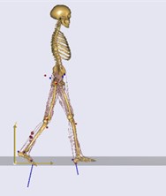
After experiment preparation you should start an experiment. The experimental subject is human, whose body parameter should be measured by rule and line (as shown in Fig. 4). Then the employee (25 years old, male, physical health) worn black clothing with multiple markers walked naturally through the pavement placed two foot force acquisition plates (as shown in Fig. 2). The six high-speed cameras record the motion trajectory of markers in the space by 100 Hz acquisition frequency. During the process, the motion coordinates of markers’ trajectory were recorded in the projection plane of each camera by two dimensional. Then six groups of two-dimensional arrays were mapped to a three-dimensional coordinate in the Cartesian coordinate system by the internal algorithm. The three-dimensional coordinate was the real position of the marker in the space. Combined with ground reaction force (GRF) measured by the foot force plate, the human joints’ torque during each gait sub phase could be calculated based on the human dynamics model.
2.2. Kinematic model based on multi-rigid body kinematics
During the process of experimental data analysis, we analyze the human motion by kinematic model based on multi-rigid body kinematics (seen in Section 2.2) and dynamic model based on Newton Euler mechanics (seen in Section 2.3).
Mathematical model of human is reconstructed by the multi rigid body kinematics. Take knee joint as an example, the triangle whose three vertexes are p3, p4, and p5 presents the shank segment (as shown in Fig. 5). The coordinates are defined by the triangle, where is the unit vector from point 3 to point 5; is the unit normal vector of the triangular plane, is determined by the right-hand rule. The expressions are as Eqs (1-3).
Fig. 43-D coordinate reconstruction
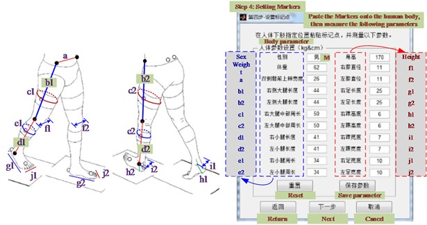
Fig. 53-D coordinate reconstruction
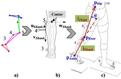
According to the empirical formula, the coordinate of the human’s knee center is derived by using the coordinates of the markers and unit vector:
where, is the width of the knee joint (as shown in Fig. 4). Similarly, the coordinates of the center of the right hip and ankle are and .
The shank and thigh segments are defined by the unit vector of the axis from the center of gravity of thigh to the center of gravity of shank:
Finally, the angle of knee joint is expressed about the two unit vector using Trigonometric equation:
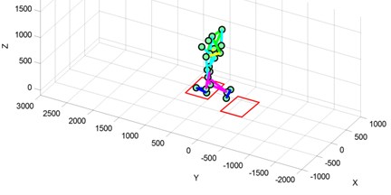
In the same way, , , , , could be achieved. The numerical values of the six angles change with human walking, whose law is shown is Section 3.2. In the experimental data analysis, we could reconstruct human walking process by driving a 3-D virtual human using the data of joints’ angle. As a result, the motion of the 3-D virtual human is very smooth, almost the same with the employee’s real gait. Therefore, the measured result can be trustworthy.
Fig. 6The reconstructed walking gait by 3-D virtual human
2.3. Dynamic model based on Newton Euler mechanics
Based on the Newton Euler mechanics, the mechanical equation was derived based on the balance equation of force and torque. According to the multi-rigid body theory, the human lower limb was divided into thigh segment, shank segment and foot segment (as shown in Fig. 7).
Fig. 7Relation of force and torque on each joint
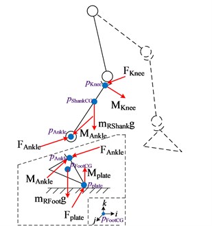
For the foot segment, the force and torque of ankle are as follows according to the Newton’s second law:
where, [0 0 –1]T, is the acceleration of , which is the center of gravity of right foot. is estimated quality by anatomical empirical formula, whose expression is = 0.0083 Weight + 254.5 – 0.065 (Weight, , and are shown in Fig. 4). And the other variables are as follows:
where, , , are the three components of , which is the first-order derivative of right foot’s angular momentum. They are solved as follows:
where, , , are velocity of right foot about coordinate axis , and , whose value are updated automatically by computer as walking gait. , , are rotational inertia of right foot about coordinate axis , and , whose value are determined by anatomical empirical equation.
According to Eqs. (10)-(13), Eq.(9) could be expressed as:
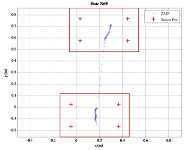
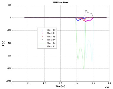
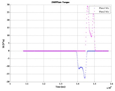
where, is zero moment point (ZMP), i.e. the the center of (as shown in Fig. 8). and are achieved by the foot force measuring system (as shown in Fig. 9). Although is a three-dimensional vector, what we concern about is the motion on the sagittal plane, i.e. the - plane. The following discussion is based on this. The experiment results of will be shown in Section 3.2.
Fig. 8Locomotion trajectory of ZMP (pplate)
As the knee joint and hip joint, the method is the same that will not be repeat here.
2.4. Muscle biomechanics simulation model
Muscles, the drive source of the joint motion, help people walk easy and acclimatize himself to kinds of complex ground comfortably, which is a sophisticated and perfect bio-actuator and pretty useful for the design and control of the exoskeleton actuator. However, muscle’s force is unable measured by test directly because muscles are distributed in body tissues complicatedly. As a result, simulation becomes an effect way [8]. The Any Body Modeling System (ABMS) is a modeling and simulation software that could analyze the mechanics of the live human body working in concert with its environment by computer-aided engineering (CAE). As the external forces and boundary conditions of environment are defined and the posture or motion for the human body is impose on from a set recorded motion data, ABMS then runs a simulation and calculates individual muscle forces, joint forces and moments, metabolism, elastic energy in tendons, antagonistic muscle actions and much more (as shown in Fig. 1).
Fig. 9Fplate and Mplate
a)
b)
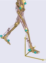
The simulation model is shown as Fig. 10. The greed balls drive the human simulation model to walk, correspond with the markers when doing a human motion capture experiment (as shown in Fig. 3). The length and quality of the simulation model are determined according to the real values of the employee, the same as Fig. 4 and Section 2. 3. When the model walks, all muscles work together to balance the external forces, including force from environment and bone gravity. In ABMS, the force of each muscle is obtained by solving the optimal solution of a target function (as Eq. (15) shows), which means to finish a work with minimal muscle activity.
where, is power number, is the muscle force of muscle and is its area. is the total number of muscle.
The constraint condition of Eq. (15) is:
Eq. (16) defines the dynamic equilibrium. Where, is coefficient matrix of muscle force, d is the vector of external forces.
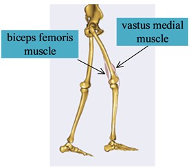
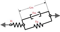
From previous research, it is found that the knee joint plays an important role in vibration reduction and swing during walk. Hidden display other muscles, only the principal muscles driving knee joint are kept for clarity, as shown in Fig. 10(b). So, the article addressed on the analysis of the knee principal muscle’s force. Around the knee joint, the biceps femoris muscle and the vastus medial muscle are a pair of antagonists, expressed by the Hill model [9] (as shown in Fig. 10(c)). presents the force generated by the contractile element, representing the active properties of the muscle fibers. is the force generated by the parallel-elastic element representing the passive stiffness of the muscle fibers. is the force generated by the serial-elastic element representing the elasticity of the tendon. is the length of the contractile element and Lt is the length of the tendon.
Fig. 10Simulation model in ABMS
a)
b)
c)
Fig. 11The main muscles around the knee joint
a)
b)
c)
When all settings are made, we can run simulation, whose simulation time is a cycle of whole walking gait, as shown in Fig. 11. The change law of muscle force for human walking would show in Section 4.
3. Experiment data of human walking gait
3.1. A whole gait
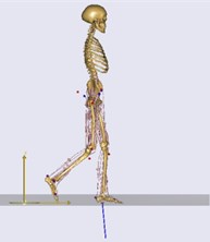
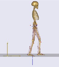
The natural gait could be roughly divided into the support phase and the swing phase. Compared with the swing phase, the support phase is more complex. According to the GRF, the support phase is divided into three sub-phases further. During the sub-phase I, the heel of the swing leg strikes the ground, and the two legs support on the ground at the same time initially, during which process the center of gravity transfers from the latter leg to the front leg gradually. During the sub-phase II, only the support leg is on the ground and the other leg swings in the air. During the sub-phase III, the original swing leg touches the ground again and the toe of the original support leg begins moving off the ground, preparing to enter the next gait cycle.
3.2. Kinematic and dynamics during the three support sub- phases
Each test is carried for three times repeatedly. The following conclusions could be drawn from Figs. 7-9. Firstly, the whole range of hip’s angle, knee’s and ankle’s were 40°~ –15°, 0°~60° and –17°~20°, respectively. Besides, the ranges of the three joints’ angle were listed as Table 4. Thirdly, all the joint torque curves were approximate sine function, among which the torque of the ankle was largest equal to the sum of knee’s and the hip’s approximately. All of the data perform has a guidance function to the motion control of exoskeleton’s joints during different sub-phases on the support phase.
Fig. 12Hip joint
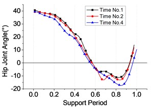
a) Angle
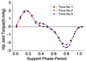
b) Torque
Fig. 13Knee joint
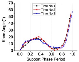
a) Angle
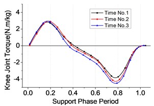
b) Torque
Fig. 14Ankle joint
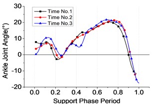
a) Angle
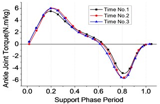
b) Torque
4. Biomechanical simulation of the main muscles around the knee joint
4.1. Vastus medialis muscle
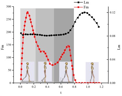
During the support phase (0-0.8 s).
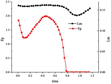
During this period, the vastus medialis muscle generated an active contraction force to stretch the knee joint and the muscle length maintained 0.08 m or so (as shown in Fig. 15) for the muscle being in isometric contraction, which lead to that was near zero (as shown in Fig. 16(a)). At this time, , so the vibration of was similar with (as shown in Fig. 15 and Fig. 16(b)). From the view of , the vastus medialis muscle got a complex vibration during sub-phase I, II and III. reached a maximum value of 280 N or so at 0.1 s during sub-phase I when the leg just touched the ground. However, when the leg entered the real support phase, i.e. sub-phase II and III, the force of the muscle decreased rapidly because the human leg could rely on its own skeleton because it was vertical to the ground.
Table 4Angle range of joints
Sub-phase | Joint | Period (s) | Range of angle (°) | ||
No.1 | No.2 | No.3 | |||
I | Hip | 0-0.2 | 36-40 | 35-39 | 33-39 |
Knee | 2-14 | 1-16 | 2-15 | ||
Ankle | –3-8 | 0-7 | 0-11 | ||
II | Hip | 0.2-0.8 | –10-36 | –12-35 | –14-33 |
Knee | 7-18 | 1-21 | 4-17 | ||
Ankle | –2-20 | –2-21 | 0-21 | ||
III | Hip | 0.8-1 | –10-13 | –12-12 | –12-10 |
Knee | 7-58 | 7-56 | 4-58 | ||
Ankle | -12-18 | –15-20 | –17-20 | ||
Fig. 15Variation curve of muscle active force Fm versus the muscle length Lm (vastus medialis muscle)
During the swing phase (0.8 s-1.2 s).
When entering the swing phase, the vastus medialis muscle was stretched passively, no more as an active unit, during which process was zero, as shown in Fig. 15. So, we addressed our research on . At this time reached a maximum value of 0.12 m. changed from small to large and then from large back to small. During the process, reached a maximum value of 100 N at the maximal bending angle of the knee joint (as shown in Fig. 16(a)).
4.2. Biceps femoris muscle
In contrast to the vastus medialis muscle, it was passive during the supporting phase and active in the swing phase.
During the support phase (0-0.8 s).
maintained an original length of 0.16 m. Meanwhile, kept zero because the biceps femoris muscle was under relaxation. The value of was very small so that it could be ignored (as shown in Fig. 18(a)).
During the swing phase (0.8 s-1.2 s).
Once entering the swing phase, the biceps femoris muscle started playing an active function. As the decrease of the knee joint’s angle, the muscle shrunken its length from 0.16 m to 0.13 m (as shown in Fig. 17). After that it slowly released back to the original length until the end of the swing phase. The active force reached a maximum of 220 N (as shown in Fig. 17). However, as we know, in the Hill model, should changes significantly as changes (because the parallel-elastic element was in parallel with the active unit, was not only the length of the active unit, but also the length of the parallel-elastic element), but from Fig. 18(a) we could found that things were not that case. Why? A reasonable explanation was that the muscle was a two-element muscle instead of a three-element muscle, i.e. the Hill model.
Fig. 16Variation curve of Fp and Ft versus the muscle length Lm (vastus medialis muscle)
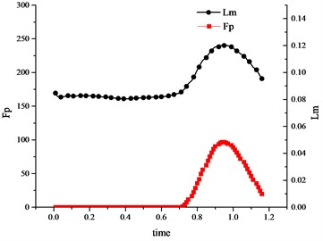
a) Muscle passive force
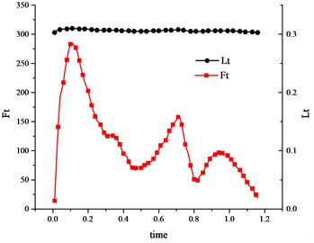
b) Tendon force
Fig. 17Variation curve of muscle active force Fm versus the muscle length Lm (biceps femoris muscle)
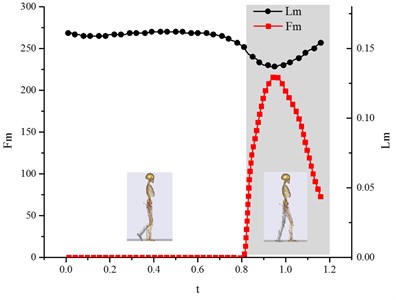
Fig. 18Variation curve of Fp and Ft versus the muscle length Lm (vastus medialis muscle)
a) Muscle passive force
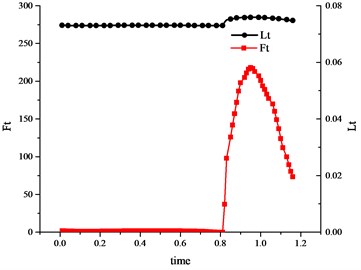
b) Tendon force
5. Conclusions
The research on the human walking motion and the activities of relevant muscles is able to supply important enlightenment to the design of the exoskeleton. For human walking gait, the multi-camera motion capture system and foot force measuring system were built, by which the kinematic and dynamic performance of three joints of lower limb were achieved. It is also important to figure out the properties of human muscles, a sophisticated and perfect bio-actuator, which has a pretty good guidance for the design and control of the exoskeleton actuator. Firstly, the kinematic and dynamic equations of human lower limb were derived by the multi-rigid body kinematics and the Newton Euler mechanics. Besides, the three-element muscle model, i.e. the Hill model, was introduced. Thirdly, by the human walking experiment, the angle curves of the three joints of the lower limb were obtained by the motion capture system. Considering that the process of the support phase was more complex than that of the swing phase, the article stressed the three sub-phases of the support phase. Fourthly, the biomechanics of the relevant muscles driving the knee joint were simulated by the human simulation soft. It was found that the vastus medialis muscle was the principal muscle during knee’s extension that could provide a maximum force of 280 Nm. In contrast, the biceps femoris muscle was the principal muscle during knee’s flexion that could provide a maximum force of 220 Nm.
In conclusion, the human body is the result of natural evolution, having a good movement forms and flexible driving mode. This article has not only achieved the kinematics and dynamics data about human lower limb by experiment, but also researched the biomechanics of the principal muscle of knee joint under walk gait. All the work explores the function of human joint actuator, in detail, i.e. muscle, which is useful for bionics design of artificial limb and exoskeleton robot.
References
-
Lee H., Kim W., Han J., et al. The technical trend of the exoskeleton robot system for human power assistance. International Journal of Precision Engineering and Manufacturing, Vol. 13, Issue 8, 2012, p. 1491-1497.
-
Zoss A. B., Kazerooni H., Chu A. Biomechanical design of the Berkeley lower extremity exoskeleton (BLEEX). IEEE-ASME Transactions on Mechatronics, Vol. 11, Issue 2, 2006, p. 128-138.
-
Kim W., Lee H., Kim D., et al. Mechanical design of the hanyang exoskeleton assistive robot (HEXAR). 14th International Conference on Control, Automation and Systems (ICCAS 2014), Korea, 2014.
-
Yali H., Xingsong W. Biomechanics study of human lower limb walking: implication for design of power-assisted robot. IEEE/RSJ International Conference on Intelligent Robots and Systems, Taipei, Taiwan, 2010.
-
Chu A., Kazerooni H., Zoss A., et al. On the biomimetic design of the Berkeley lower extremity exoskeleton (BLEEX). IEEE International Conference on Robotics and Automation, 2005, p. 4345-4352.
-
Seo Changhoon, Kim Hong Chul, Wang Ji Hyeun Lower-limb exoskeleton testbed for level walking with backpack load. Journal of the Korea Institute of Military Science and Technology, Vol. 18, Issue 3, 2015, p. 309-315.
-
Han Y. L., Wang X. S. The biomechanical study of lower limb during human walking. Science China: Technological Sciences, Vol. 5, 2011, p. 983-991.
-
Wu J. Z., An K., Cutlip R. G., et al. Modeling of the muscle/tendon excursions and moment arms in the thumb using the commercial software anybody. Journal of Biomechanics, Vol. 42, Issue 3, 2009, p. 383-388.
-
Smith P. N., Refshauge K. M., Scarvell J. M. Development of the concepts of knee kinematics. Archives of Physical Medicine and Rehabilitation, Vol. 84, Issue 12, 2003, p. 1895-1902.
About this article

