Path tracking control for inverse problem of vehicle handling dynamics

Liu, Yingjie; Cui, Dawei; Fu, Yu

doi:10.21595/jve.2017.18342

Journal of Vibroengineering

Browse Journal

Submit article

Published: 30 September 2017

Check for updates

Path tracking control for inverse problem of vehicle handling dynamics

Yingjie Liu¹

Dawei Cui²

Yu Fu³

^{1, 2}School of Mechanical-Electronic and Vehicle Engineering, Weifang University, Weifang, 261061, Shandong, China

³College of Aeronautical Engineering, Civil Aviation University of China, Tianjin, 300300, China

Corresponding Author:

Yingjie Liu

Cite the article Download PDF

Downloads 1746

WoS Core Citations 1

CrossRef Citations 2

Abstract

A path tracking controller based on active disturbance rejection control(ADRC) theory is presented in this paper to solve path tracking problem in inverse vehicle handling dynamics. The basic idea behind the work is to design an active disturbance rejection controller according to yaw rate and lateral displacement during a vehicle travels along a prescribed path to generate an expected trajectory which guarantees minimum clearance to the prescribed path. Aiming at this purpose, using preview follower theory, a linear extended state observer based on lateral displacement is designed. Considering yaw angle of vehicle, a non-linear combination function combined error of lateral displacement as well as error of yaw angle is designed according to monotone bounded hyperbolic of tangent function. Finally, a real vehicle test is executed to verify the rationality of the path tracking controller. At the same time, according to characteristics of pavement file in Carsim, a 3-D virtual pavement model is established and ride comfort simulation of random pavement is carried out in the software model. The results show that the minimum lateral position error of the generated path tracking trajectory can be good indicators of successful solving of the path tracking problem in inverse vehicle handling dynamics for ADRC. More precisely, there is higher calculation accuracy for the algorithm of the ADRC to solve the path tracking problem. The study can help drivers easily identify safe lane-keeping trajectories and area.

1. Introduction

The emergence of automobile has brought great changes to human life style. The rapid development of automobile industry and the continuous improvement of economic level have brought not only popularization of automobile but also a series of social problems. As a result, road traffic accidents have become serious global public safety problems. The growing mobility of people and goods has a very high societal cost in order to protect people from vehicle accidents. Most car accidents occur because of human mistakes in decision making and vehicle handling of the vehicle. Several studies show that the driver is responsible for most accidents, which occur mainly due to distraction and wrong perception and judgment of the traffic and environmental situations around the vehicle. As autonomous vehicles enter public roads, they must be capable of not only normal driving but also maneuvers to avoid accidents [1-7].

These accidents can be avoided by certain vehicle control systems, particularly an active safety control system. The development of advanced active safety systems that improve vehicle stability is a prominent area of automotive research.

The path tracking problem has been studied in the literatures. A brief review is presented in what follows.

Luo, et al. [8], designed a dynamic automated lane change maneuver based on vehicle-to-vehicle communication to accomplish an automated lane change and eliminate potential collisions during the lane change process. Esmaeil, et al. [9], presented a Fuzzy Inference System (FIS) which models a driver’s binary decision to or not to execute a discretionary lane changing move on freeways. Wu, et al. [10], proposed a novel modeling and simulation environment developed under Matlab/Simulink with friendly and intuitive graphic user interfaces, aimed to enable math-based virtual development and test of intelligent driving systems. Miyake, et al. [11], considered a function that displays lane guidance on an image of the front scene that matches what drivers actually see outside the vehicle in order to achieve intuitive lane guidance. Hou, et al. [12], developed a lane changing assistance system that advises drivers of safe gaps for making mandatory lane changes at lane drops. Desiraju, et al. [13], proposed an algorithm which is distributed in nature and made use of vehicle-to-vehicle and/or vehicle-to-infrastructure communication technologies to judiciously make local lane-change decisions while guaranteeing that no collisions will occur. Dang, et al. [14], designed a novel coordinated ACC system with a lane-change assistance function, which enables dual-target tracking, safe lane change, and longitudinal ride comfort. The paper analyzed lane-change risk by calculating minimum safety spacing between the host vehicle and surrounding vehicles and developed a coordinated control algorithm using model predictive control theory. Wang, et al. [15], proposed a multiple cycle sine-wave steering input (MCSSI) maneuver to solve the single lane-change maneuvers problem exploring the effect of the transient response. Benloucif, et al. [16], presented an automated driving system that is structured in hierarchical levels to allow suitable interaction with the driver on multiple driving levels to ensure cooperation with the driver. Yan, et al. [17], developed driver’s trust in assistance systems based on the assumption that driver’s appropriate trust in these systems can be built when the support of assistance systems is adapted to the drivers’ uncertainty state and helps reducing their uncertainty.

The above method can solve the path tracking problem effectively but has some drawbacks such as difficulty in rule-making, strong dependency on precision of model of the controlled object and insufficient consideration of external disturbance.

This paper aims to present a controller based on active disturbance rejection control theory for path tracking problem in inverse vehicle handling dynamics. The method is used to build the active disturbance rejection controller for vehicle tracking the desired path with optimal control input. Focusing on the above purpose, this paper presents a 3-DOF vehicle model and then proposes the active disturbance rejection controller for path tracking problem. Taking into account the effectiveness of the proposed method, we propose a comparative verification. After verifying correctness of the numerical simulation by experiment, the conclusions are summarized and the future research directions are suggested.

2. Model of vehicle path tracking problem

2.1. Mathematical model of vehicle path tracking problem

It is assumed that the influence on the steering system，suspension，unevenness of road and air resistance is ignored, and the steering angle at the front wheels is set as input. The vehicle movement can be simplified as a 3-DOF vehicle model which can reflect the lateral dynamics of the vehicle depicted accurately in Fig. 1. For simplicity, in order to make the design of the path tracking controller meet the demand of engineering applications the controller is designed based on the 3-DOF vehicle model.

The dynamics equation of the 3-DOF vehicle model can be described as:

1

\{\begin{array}{l} m a_{y} = 2 F_{y f} + 2 F_{y r} + F_{b a n k}, \\ I_{z} \dot{γ} = 2 l_{f} F_{y f} - 2 l_{r} F_{y r}, \end{array}

where $m$ is vehicle mass; $I_{z}$ is yaw moment of inertia; $l_{f}$ and $l_{r}$ are the distances of center of gravity of the vehicle to the front and rear axles, respectively; $a_{y}$ is lateral acceleration of the vehicle; $F_{y f}$ and $F_{y r}$ are the lateral forces generated in the tires; $F_{b a n k}$ is the force generated as a result of bank angle. The bank angle is ignored hence and $F_{b a n k}$ is set to zero; $γ$ is the yaw rate.

Fig. 13-DOF vehicle model

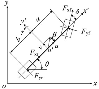
To calculate the vehicle positions in the Earth coordinate defined by $x$ and $y$ , the vehicle velocity in the body coordinate is projected in the Earth coordinate as:

\{\begin{array}{l} \dot{x} = u c o s θ - v s i n θ, \\ \dot{y} = v c o s θ + u s i n θ, \end{array}

where $θ$ is the heading angle of the vehicle.

2.2. Tire model

The lateral force which is calculated by the linear tire model is required to complete obstacle-avoidance maneuver by steering. And the lateral stiffness of the tire is estimated based on the Magic equation tire model. It is assumed that the load transfer is ignored, and the left sideslip angle of the tire is equal to the right one. The lateral forces of front and rear wheels can be expressed as:

2

\{\begin{array}{l} F_{y f} = c_{f} α_{f}, \\ F_{y r} = c_{r} α_{r}, \end{array}

where $c_{f}$ and $c_{r}$ are the lateral stiffness of the front and rear tires. $α_{f}$ and $α_{r}$ are the front and rear slip angles. $c_{f}$ and $c_{r}$ are estimated by the initial slope of Magic equation tire model:

3

\{\begin{array}{l} c_{f} = \frac{\partial F_{y f}}{\partial α_{f}}| α_{f} = 0, \\ c_{r} = \frac{\partial F_{y r}}{\partial α_{r}}| α_{r} = 0 . \end{array}

Constrains on the slip angle of front and rear tires as well as the side slip angel and the yaw rate are imposed as:

4

\{\begin{array}{l} α_{f} = β + \frac{l_{f} γ}{u} - δ, \\ α_{r} = β - \frac{l_{r} γ}{u}, \end{array}

where $β$ is the side slip angle; $u$ is the longitudinal velocity; $δ$ is the front steering angle.

In state space form the basic equation of motion for this model is:

5

[\begin{array}{l} \dot{β} \\ \dot{γ} \end{array}] = [\begin{matrix} - \frac{c_{f} + c_{r}}{m u} & - 1 - \frac{l_{f} c_{f} - l_{r} c_{r}}{m u^{2}} \\ - \frac{l_{f} c_{f} - l_{r} c_{r}}{I_{z}} & - \frac{l_{f}^{2} c_{f} + l_{r}^{2} c_{r}}{I_{z} u} \end{matrix}] [\begin{array}{l} β \\ γ \end{array}] + [\begin{array}{l} \frac{c_{f}}{m u} \\ \frac{l_{f} c_{f}}{I_{z}} \end{array}] δ .

2.3. Optimal preview time

A small preview time $T$ will make amplitude of the steering angle increased as well as the steering rate in the path tracking process. So, the errors between the tracking path and the ideal path will become smaller as a result. But too small preview time will lead to instability or even oscillation for the system.

The preview time was calculated by experimental calibration methods in the past. A large preview time will make the difference between the tracking path and the ideal path become larger but can reduce the steering angle as well as the steering rate as well as reducing the lateral acceleration of the vehicle.

The preview time should be selected according to the actual driving conditions, the error between the tracking path and the ideal path $E$ and steering rate $δ_{s w}^{'}$ as well as the lateral acceleration $a_{y}$ . Comprehensive evaluation indicators which are described as following are used to solve the optimal preview time [18]:

6

\begin{array}{l} J_{T} = J_{E} + J_{{δ'}_{s w}} + J_{a_{y}} = \frac{1}{t_{n}} \int_{0}^{t_{n}} [{(\frac{E}{\hat{E}})}^{2} + {(\frac{δ_{s w}^{'}}{{\hat{δ}}_{s w}^{'}})}^{2} + {(\frac{a_{y}}{{\hat{a}}_{y}})}^{2}] d t, \end{array}

where:

7

\{\begin{array}{l} J_{E} = \frac{1}{t_{n}} \int_{0}^{t_{n}} {(\frac{E}{\hat{E}})}^{2} d t, \\ J_{{δ'}_{s w}} = \frac{1}{t_{n}} \int_{0}^{t_{n}} {(\frac{δ_{s w}^{'}}{{\hat{δ}}_{s w}^{'}})}^{2} d t, \\ J_{a_{y}} = \frac{1}{t_{n}} \int_{0}^{t_{n}} {(\frac{a_{y}}{{\hat{a}}_{y}})}^{2} d t . \end{array}

where $t_{n}$ is the duration in the path tracking processing; $J_{E}$ , $J_{{δ'}_{s w}}$ and $J_{a_{y}}$ are evaluation indicators of the error between the tracking path and the ideal path $E$ and steering rate $δ_{s w}^{'}$ as well as the lateral acceleration $a_{y}$ respectively. $\hat{E}$ , ${\hat{δ}}_{s w}^{'}$ and ${\hat{a}}_{y}$ are threshold values of $E$ , $δ_{s w}^{'}$ and $a_{y}$ respectively. According to [19] and the research objective of this paper, in the case of stricter constraint for the error between the tracking path and the ideal path, $E$ and $δ_{s w}^{'}$ as well as $a_{y}$ should be set as $\hat{E} =$ 0.2 m, ${\hat{δ}}_{s w}^{'} =$ 360 °/s, ${\hat{a}}_{y} =$ 0.3 g respectively. In order to solve the preview time, $J_{T}$ should be minimized.

3. Design of linear active disturbance rejection controller based on vehicle yaw rate

The Laplace variation of the state equation of the 3-DOF vehicle dynamics model is operated. Then the equation of the transfer function between yaw rate and front steering angle is obtained [20]:

8

\frac{γ (s)}{δ_{f} (s)} = \frac{d s + e}{a s^{2} + b s + c},

where:

\begin{array}{l} a = m u I_{z}, b = m (l_{f}^{2} c_{f} + l_{r}^{2} c_{r}) + I_{z} (c_{f} + c_{r}), \\ c = c_{f} c_{r} (l_{f} + l_{r})^{2} / u - m u (l_{f} c_{f} - l_{r} c_{r}), \\ d = m u c_{f} l_{f}, e = c_{f} c_{r} (l_{f} + l_{r}) . \end{array}

Eq. (9) can be obtained by implementing Laplace inverse transformation on Eq. (8):

9

\ddot{γ} = - \frac{b}{a} \dot{γ} - \frac{c}{a} γ + \frac{d}{a} {\dot{δ}}_{f} + \frac{e}{a} δ .

It is assumed that $γ = x_{1}$ , $\dot{γ} = x_{2}$ , $\ddot{γ} = {\dot{x}}_{2}$ , $b_{0} = e / a$ then Eq. (10) can be expressed as:

10

f [x_{1}, x_{2}, {\dot{δ}}_{f}] = - \frac{b}{a} \dot{γ} - \frac{c}{a} γ + \frac{d}{a} \dot{δ} .

Eq. (10) can be transformed into an integrator-series system. More precisely, that is the standard form:

11

\{\begin{array}{l} {\dot{x}}_{1} = x_{2}, \\ {\dot{x}}_{2} = f (x_{1}, x_{2}, \dot{δ}) + b_{0} δ \\ y = x_{1} . \end{array},

According to the second-order integrator series system shown in Eq. (11), a second-order linear active disturbance rejection path tracking controller based on yaw rate is designed as shown in Fig. 2.

Fig. 2Second-order linear ADRC of path tracking

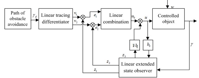
From Fig. 2 it can be seen that the linear active disturbance rejection controller consists of three parts: a linear tracing differentiator, a linear combination and a linear extended state observer. The linear tracking differentiator which is capable of arranging a transition process for reference input signal and extracting first-derivative of the ideal input signal and filter input signals $γ_{d}$ is located in the feed-forward link of the linear active disturbance rejection controller. And the tracking differentiator is a non-linear dynamic link. The core component of the linear active disturbance rejection controller is the linear extended state observer, which can estimate the external disturbance and the model uncertainty in real time and compensate in the feedback control. Outputs ( $z_{1}$ , $z_{2}$ ) of the linear extended state observer and the tracking signals ( $v_{1}$ , $v_{2}$ ) of the linear tracking differentiator can provide the control law ( $u_{0}$ ) operating on the actuator of the controlled object by the linear combination of the error ( $e_{1}$ ) and the differential ( $e_{2}$ ) of the error.

The discretization of each part of the expression is as follows:

(1) Linear tracing differentiator:

12

\{\begin{array}{l} v_{1} (k + 1) = v_{1} (k) + h v_{2} (k), \\ v_{2} (k + 1) = v_{2} (k) + h [- k_{1} (v_{1} (k) - γ_{d} (k)) - k_{2} v_{2} (k)], \end{array}

where $γ_{d} (k)$ is the target input signal; $h$ is the simulation step length; $k$ is the number of samples; $v_{1} (k)$ and $v_{2} (k)$ track $γ_{d} (k)$ and ${\dot{γ}}_{d} (k)$ respectively; $k_{1}$ and $k_{2}$ are design parameters.

(2) Linear extended state observer:

13

\{\begin{array}{l} e (k) = z_{1} (k) - γ (k), \\ β_{01} = 3 ω_{0}, β_{02} = 3 ω_{0}^{2}, β_{03} = ω_{0}^{3}, \\ z_{1} (k + 1) = z_{1} (k) + h [z_{2} (k) - β_{01} e (k)], \\ z_{2} (k + 1) = z_{2} (k) + h [z_{3} (k) - β_{02} e (k) + b_{0} u (k)], \\ z_{3} (k + 1) = z_{3} (k) + h [- β_{03} e (k)], \end{array}

where $γ (k)$ is output of the controlled object; $z_{1} (k)$ , $z_{2} (k)$ and $z_{3} (k)$ are outputs of the linear extended state observer; $ω_{0}$ is bandwidth of the linear extended state observer; $b_{0}$ is design parameter.

(3) Linear combination:

14

\{\begin{array}{l} e_{1} (k + 1) = v_{1} (k + 1) - z_{1} (k + 1), \\ e_{2} (k + 1) = v_{2} (k + 1) - z_{2} (k + 1), \\ β_{1} = \frac{2 ω_{c}}{b_{0}}, β_{2} = \frac{ω_{c}^{2}}{b_{0}}, \\ u_{0} (k + 1) = β_{1} e_{1} (k + 1) + β_{2} e_{2} (k + 1), \end{array}

where $ω_{c}$ is desired bandwidth of the closed-loop system, $ω_{0} =$ 5-10 $ω_{c}$ . $β_{1}$ and $β_{2}$ are design parameters which are solved by bandwidth of the closed-loop system.

The control law ( $u_{0}$ ) is a linear combination of the error ( $e_{1}$ ) and the differential ( $e_{2}$ ) of the error. The unknown disturbance should be eliminated before the actuator of the controlled object is input. The control ( $u$ ) operating on the actuator of the controlled object can be expressed as:

15

u (k + 1) = u_{0} (k + 1) - \frac{z_{3} (k + 1)}{b_{0}} .

4. Numerical simulation and experimental verification

4.1. Simulation result

In order to verify the control effect of the path tracking controller, simulation is carried out by Carsim/Simulink. Carsim which is one kind of vehicle dynamics simulation software can simulate the real vehicle dynamic characteristics and analyze vehicle response to driving control on different 3-D pavements as well as having the advantages of convenient rapid operation and high simulation precision.

Fig. 3 shows the co-simulation of Carsim and Simulink.

In order to compare with results of real vehicle test, simulation parameters of the simulation should be consistent with parameters of a certain real vehicle. And the parameters of the real vehicle used in the simulation are shown in Table 1.

Fig. 3Block diagram of co-simulation

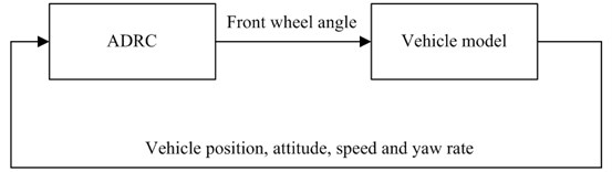
Fig. 4Double lane change test road (● stands for stake)

The tracked path is prescribed as the double lane change test road shown in Fig. 4, where $s_{0} = s_{1} = s_{2} = s_{4} = 2 u,$ $s_{3} = u$ , $s_{5} = 5 u$ , $s_{6} = 3 u$ . $B$ is the lane change distance, $B =$ 3.5 m. $B_{1},$ $B_{2}$ and $B_{3}$ are the distances between the stakes, $B_{1} = 1.1 L + 0.25 =$ 2.12 m, $B_{2} = 1.2 L + 0.25 =$ 2.29 m, $B_{3} = 1.3 L + 0.25 =$ 2.46 m, where $L$ is the width of the vehicle, $L =$ 1.7 m.

In realistic driving process, drivers’ ideal target trajectory should be low-level continuous smooth curve shown in Fig. 5. And also, according to ISO/TR3888-2004, the trajectory of the vehicle traveling along the pylon course slalom test road should be described as a curve of order three with continuous first-order derivative transformed with cubic splines fitting:

16

f (x) = \{\begin{array}{l} 0, & x \in s_{1}, \\ e_{0} + e_{1} x + e_{2} x^{2} + e_{3} x^{3}, & x \in s_{2}, \\ B, & x \in s_{3}, \\ {e'}_{0} + {e'}_{1} x + {e'}_{2} x^{2} + {e'}_{3} x^{3}, & x \in s_{4}, \\ 0, & x \in s_{5}, \end{array}

where:

a_{0} = s_{1}, a_{1} = s_{1} + s_{2}, a_{2} = s_{1} + s_{2} + s_{3}, a_{3} = s_{1} + s_{2} + s_{3} + s_{4}, d = a_{1} - a_{0},

d^{'} = a_{2} - a_{3}, e_{0} = a_{0}^{2} (3 a_{1} - a_{0}) B / d^{3}, e_{1} = - 6 a_{0} a_{1} B / d^{3}, e_{2} = 3 (a_{0} + a_{1}) B / d^{3},

e_{3} = - 2 B / d^{3}, e_{0}^{'} = a_{3}^{2} (3 a_{2} - a_{3}) B / d'^{3}, e_{1}^{'} = - 6 a_{3} a_{2} B / d'^{3},

e_{2}^{'} = 3 (a_{3} + a_{2}) B / d'^{3}, e_{3}^{'} = - 2 B / d'^{3} .

Fig. 5Fitted double lane change test road

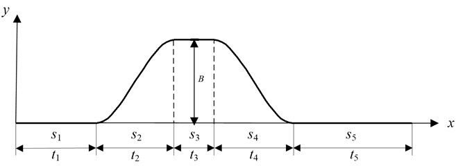
Table 1Simulation parameters

Parameter	Symbol	Value	Unit
Vehicle mass	$m$	1265	kg
Yaw moment of inertia	$I_{z}$	1800	kg·m²
Distances of center of gravity to the front axle	$l_{f}$	1.170	m
Distances of center of gravity to the rear axle	$l_{r}$	1.195	m
Steering gear ratio	$i$	20
Front wheel roll stiffness	$C_{φ 1}$	60544	N·m/rad
Rear wheel roll stiffness	$C_{φ 2}$	32750	N·m/rad
Lateral stiffness of the front tires	$c_{f}$	40021	N/rad
Lateral stiffness of the rear tires	$c_{r}$	74648	N/rad
Height of the center gravity	$h_{g}$	0.53	m

From Eq. (16) it is easy to obtain the relationship between $y$ , i.e. $f (x)$ and $x$ by substituting $t$ with $x / u$ :

17

f (t) = \{\begin{array}{l} 0, & t \in t_{1}, \\ g_{0} + g_{1} t + g_{2} t^{2} + g_{3} t^{3}, & t \in t_{2}, \\ b, & t \in t_{3}, \\ h_{0} + h_{1} t + h_{2} t^{2} + h_{3} t^{3}, & t \in t_{4}, \\ 0, & t \in t_{5}, \end{array}

where: $g_{0} = e_{0}$ , $g_{i} = e_{i} u^{j}$ ( $j =$ 1, 2, 3), $h_{0} = e_{0}^{'}$ , $h_{i} = e_{i}^{'} u^{j}$ ( $j =$ 1, 2, 3).

In order to verify the control effect of ADRC based on vehicle yaw rate, the vehicle longitudinal speed is set as $v =$ m/s and the road adhesion coefficient is set as $μ =$ 0.8 in the process of path tracking. The value of the optimum pre-sighting time is 1.06 s. And the parameters of the auto disturbance rejection path-tracking controller are: $h =$ 0.001, $k_{1} =$ 19, $k_{2} =$ 10, $ω_{0} =$ 300, $ω_{c} =$ 50, $b_{0} =$ 341.

Fig. 6Lateral distance

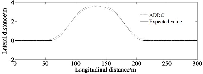
Fig. 6 shows the result of the lateral distance throughout the process of tracking the double lane change test road. It can be seen from the figure that the vehicle can track the double lane change test road well with an initial speed of 105 km/h verifying good control effect of auto-disturbance rejection controller based on vehicle yaw rate.

Fig. 7 describes the calculation result of the absolute error between the simulation result of the lateral distance and the prescribed path. It can be seen from the figure that the maximum lateral displacement error is less than 0.11 m in the whole process of path tracking. It indicated that the vehicle can track the ideal planning path precisely based on the auto-disturbance rejection controller.

Fig. 8 shows the result of the yaw rate of the vehicle. From the figure, it can be found that the real yaw rate curve can track the ideal yaw rate curve without overshoot quickly.

Fig. 7Absolute error of lateral distance

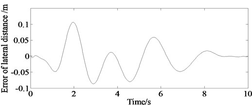
Fig. 8Simulations of yaw rate of the vehicle; solid line represents simulation value of the yaw rate controlled by ADRC, and dashed line represents expected ideal yaw rate

Simulations of yaw rate of the vehicle; solid line represents simulation value of the yaw rate controlled by ADRC, and dashed line represents expected ideal yaw rate

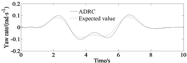
Fig. 9 describes the calculation result of the lateral acceleration. From the figure, it is shown that the lateral acceleration has bigger response values at 2.5 s, 3.8 s, 5.5 s and 7 s, which indicates that the vehicle will yield bigger lateral acceleration when it enters and moves away from the described path.

Fig. 9Simulations of lateral acceleration of the vehicle; solid line represents simulation value of the lateral acceleration controlled by ADRC, and dashed line represents expected ideal lateral acceleration

Simulations of lateral acceleration of the vehicle; solid line represents simulation value of the lateral acceleration controlled by ADRC, and dashed line represents expected ideal lateral acceleration

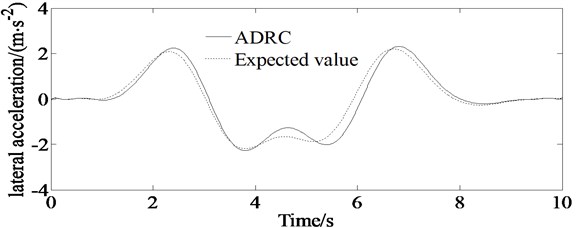
Fig. 10Simulations of steering wheel angle of the vehicle; dashed line represents simulation value of the steering wheel angle controlled by ADRC, and solid line represents expected ideal steering wheel angle

Simulations of steering wheel angle of the vehicle; dashed line represents simulation value of the steering wheel angle controlled by ADRC, and solid line represents expected ideal steering wheel angle

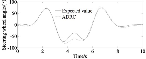
Fig. 10 describes the calculation result of the steering wheel angle. From the figure, it is shown that the steering wheel angle has bigger response values at 2.5 s, 3.8 s, 5 s and 7 s, which indicates that the vehicle needs bigger steering wheel angle when it enters and moves away from the described path.

4.2. Evaluation of calculation accuracy

From the lateral displacement error curve in Fig. 11(a), it can be concluded that the auto-disturbance rejection controller based on vehicle yaw angle is superior to the LQR-based path tracking controller. And responding speed of the ADRC controller is bigger than the LQR controller. From Fig. 11(b), it can be concluded that the maximum value of the front steering angle based on the auto-disturbance rejection controller is less than that of the LQR controller. More clear description of the evaluation of the calculation accuracy is shown in Table 2.

Fig. 11Evaluation of calculation accuracy

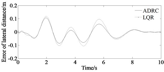
a) Simulations of error of lateral distance between the actual trajectory and expected trajectories; solid line represents simulation value of the error of lateral distance controlled by ADRC, and dashed line represents simulation value of the error of lateral distance controlled by LQR

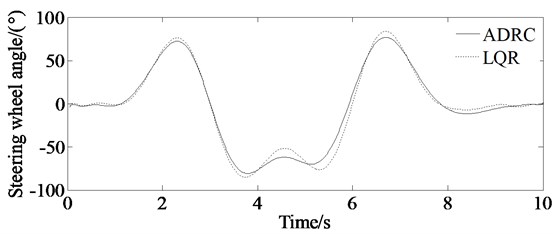
b) Simulations of steering wheel angle of the vehicle; solid line represents simulation value of the steering wheel angle controlled by ADRC, and dashed line represents simulation value of the steering wheel angle controlled by LQR

Table 2Evaluation of the calculation accuracy

Calculation results	Maximum value (absolute value)
Calculation results	ADRC	LQR
Error of lateral distance (m)	0.11	0.14
Steering wheel angle (°)	75	85

So, it is proved that there is higher control effect for the auto-disturbance rejection controller to solve the path tracking problem comparing with other traditional methods.

4.3. Experimental result

High-speed vehicle test is very dangerous. Therefore, in this paper, a model car based on a real type is simulated for the path tracking control problem and then verified by the real vehicle test.

4.3.1. Test objectives

The double lane change test is operated to obtain the longitudinal and lateral velocity, yaw rate, lateral acceleration and other test data in order to verify the correctness of the proposed algorithm.

4.3.2. Block diagram of test system and measurement equipment

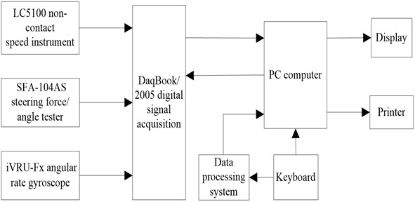
The block diagram of test system is shown in Fig. 12.

Fig. 12Block diagram of test system

4.3.3. Measurement equipment

The measurement equipment is described as following:

(1) LC5100 non-contact speed instrument and LC-1100 space filter speed sensor (shown in Figs. 13(a)-13(b)).

The LC-5100 non-contact speed instrument system is one kind of high-precision vehicle speed measurement system. The system is consisted of the LC-5100 speed tester host, LC-1100 space filter speed sensor, external speed displayer, remote control box and other components.

(2) SFA-104AS steering torque/angle tester (shown in Fig. 13(c)).

SFA-104AS steering torque/angle tester is the instrument of measuring steering torque and steering angle. The range of steering force measurement is ±98 N·m and the range of steering angle measurement is ± 1440°.

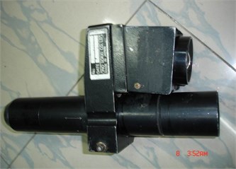
(3) iVRU-Fx angular rate gyroscope (shown in Fig. 13(d)).

The iVRU-Fx angular rate gyroscope manufactured by iMAR Company is used to measure the yaw rate, lateral acceleration and so on.

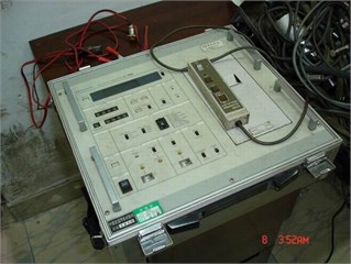
(4) DaqBook/2005 digital signal acquisition (shown in Fig. 13(e)).

The DaqBook/2005 digital signal acquisition system, manufactured by IOtech Company, USA, has a built-in 16-bit 200 kHz A/D converter with 256 analog channels and 200 K sample rate.

(5) Compaq computer (shown in Fig. 13(f)).

The Compaq computer is used to display, record and save the collected data signal.

(6) Batteries, wires and other test aids.

4.3.4. Test procedure

The test procedure in accordance with ISO/TR3888-2004 is as follows:

Step 1: Arranging stakes shown in Fig. 4 and painting prescribed path on the ground according to the double lane change test road exactly.

Step 2: Equipping the related equipment and then powering them so as to warm them up to normal operating temperature.

Step 3: With an initial velocity of 108 km/h, the tested vehicle travels along the initial lane. And then, the tested vehicle implements a lane change maneuver to another lane rapidly and then returns to the initial lane as soon as possible without touching any part of the stakes. At the same time, the time history curves of the measured variables are recorded.

Step 4: Repeating Step 3 process 12 times.

The test values are shown in Figs. 14(a)-14(d). From Figs. 14(a)-14(d) it is shown that there are errors between the simulation value and the experimental value.

Fig. 13Measurement equipments

a) LC5100 non-contact speed instrument

b) LC-1100 space filter speed sensor

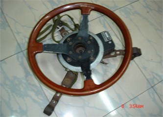
c) SFA-104AS steering torque/angle tester

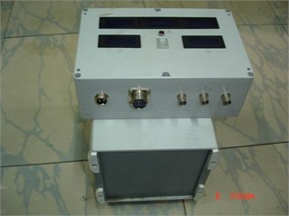
d) iVRU-Fx angular rate gyroscope

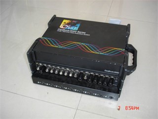
e) DaqBook/2005 digital signal acquisition

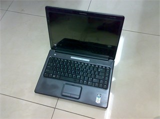
f) Compaq computer

The reasons are as following:

The drivers’ subjective feelings and driving skills are different, resulting in different responses to each driver. For example, it is shown from Fig. 14(d) that it takes about 1 second for the driver to response to track the described trajectory. At the same time, the speed for the real vehicle test is higher, so there are psychological problems performing a certain impact on the test results for the driver driving the vehicle. For example, form Figs. 14(a)-14(d) it can be seen that almost every peak of the test value (absolute value) is bigger than that of the simulation value. This is because the driver must execute bigger lateral acceleration and yaw rate as well as steering wheel angle to track the described path with higher speed. And also, there are some errors for the test equipment resulting to differences between test and simulation results.

However, the simulation value is consistent with the experimental value. So, the results shown in Figs. 14(a)-14(d) can verify the correctness of the proposed algorithm.

Fig. 14Comparison of simulation and test value

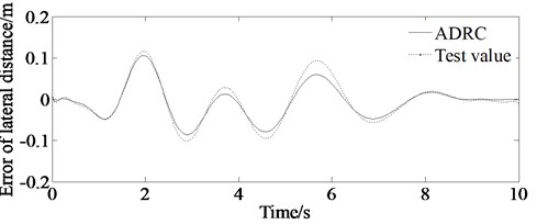
a) Error of lateral distance

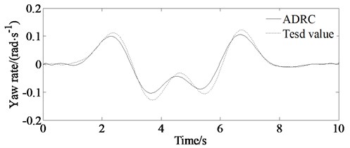
b) Yaw rate

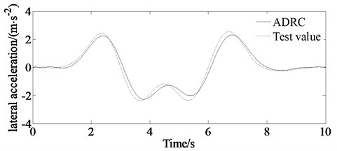
c) Lateral acceleration

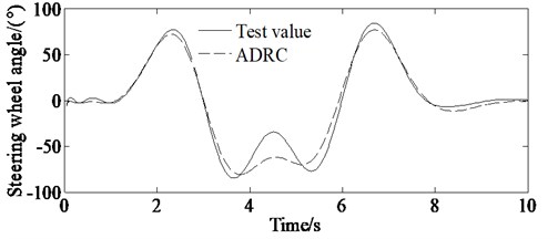
d) Steering wheel angle

4.4. Controller robustness verification in external disturbance environment

There is external interference in the process of obstacle avoidance for a vehicle with high speed. So, it is necessary to verify the control effect of the ADRC. Carsim can simulate real vehicle dynamic characteristics and can set the lateral interference and other external interference environment easily. In this paper, a C-Class Hatchback model provided by Carsim is used for control effect verification.

It is assumed that the vehicle is traveling with a longitudinal velocity of 30 m/s and an adhesion coefficient of 0.8. The parameters of the ADRC are set as $r =$ 120, $h =$ 0.001, $b_{0} =$ 15, $k_{1} =$ 19, $k_{2} =$ 10, $β_{1} =$ 1.5, $β_{2} =$ 2. The maximum speed of wind is set as 50 km/h. The step gust is shown in Fig. 15.

Fig. 16 shows the path-tracking effect when the vehicle is disturbed by lateral wind. It can be seen from Fig. 16 that ADRC can track path well according to the ideal path even there is lateral wind interference.

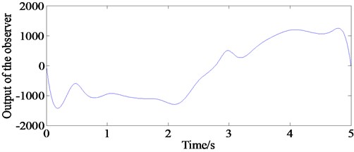
The lateral wind disturbance can be observed by the extended state observer shown in Fig. 17. It can be seen that the ADRC can compensate external interference to achieve system robustness requirements.

Fig. 15Step gust

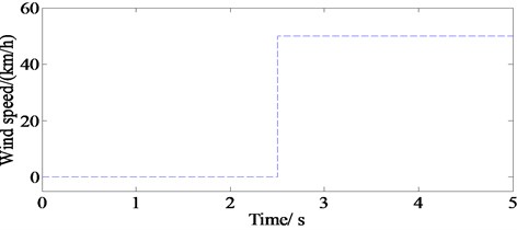
Fig. 16Lateral distance in external disturbance environment

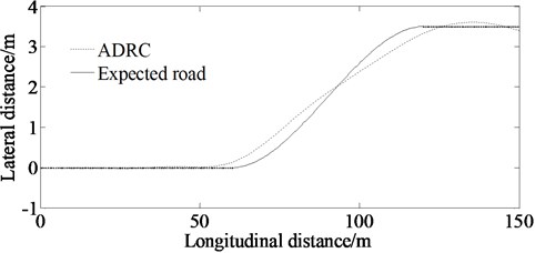
Fig. 17Output of the extended state observer

5. Rebuilding of road model and vehicle simulation of ride comfort based on Carsim

5.1. Road model

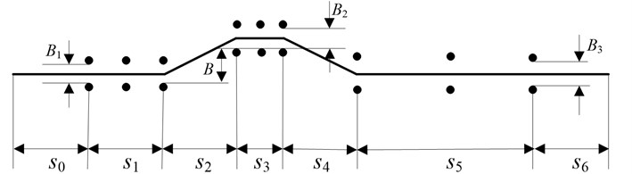
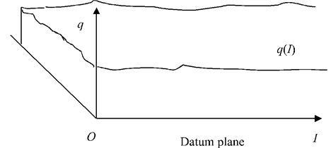
Road in Carsim is a 3-D entity. Its centerline is a spatial curve. The horizontal line of the road is a combination of straight lines, circular curves and transition curves. The longitudinal section of the road is composed of straight lines and vertical curves. The road surface is not a smooth plane. The change $q (I)$ which is road surface relative to the height of the reference plane ( $q$ ) changing along the road length $I$ is called the road roughness function shown in Fig. 18.

Road model in Carsim software is a 3-D structure and it uses the S-L-Z coordinate system. Different simulation software is corresponding to different file formats. In order to reconstruct the pavement model in Carsim, it is necessary to pave road data to write pavement file accordance with format of pavement model database.

Fig. 18Road profiling

5.2. Vehicle model in Carsim

The virtual prototype is established in Carsim. During the modeling process, the vehicle's driveline, steering and braking systems as well as the tire model are set by the default settings of Carsim. The main parameters of the test vehicle are shown in Table 1.

5.3. Simulation result

In order to verify the vehicle ride comfort, simulation of the virtual sample vehicle is carried out with an initial speed of 80 km/h by Carsim in the C-class road conditions. The simulation results are shown in Figs. 19-20. Figs. 19-20 indicate that it is effective establishing accurate 3-D road and vehicle model to evaluate vehicle ride comfort in the CarSim software providing an effective method for the dynamic performance of vehicle especially for the cooperative optimization of vehicle control ability/stability and ride comfort for further study.

Fig. 19Simulation of vertical acceleration of the centroid

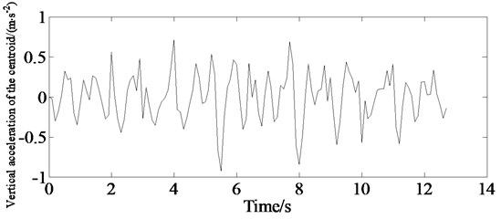
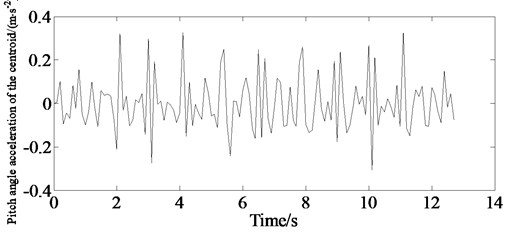
Fig. 20Simulation of pitch angle acceleration of the centroid

5.4. Experimental result

In order to verify the correctness of the simulation results, real vehicle test is carried out. In the test, a three-direction acceleration sensor (PCB-480B21 made in the USA) is placed on driver’s seat shown in Fig. 21(a). At the same time, a piezoelectric acceleration sensor is installed on body above the right front wheel of the vehicle shown in Fig. 21(b). The acceleration signal is transmitted to the tape recorder (TEACMR-30C, made in the USA) via a charge amplifier to record the acceleration signal.

Fig. 21Measurement equipment for verification of ride comfort

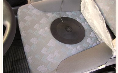
a) Three-direction acceleration sensor

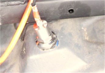
b) Piezoelectric acceleration sensorv

The test values are shown in Fig. 22. From Fig. 22 it is shown that there are errors between the simulation value and the experimental value. The main causes of the error are as following:

(1) There is difference between the pavement model and the actual road surface.

(2) The vehicle model only takes into account the simplified model established by ride comfort simulation, and there is a difference with the real vehicle, which will affect the simulation results.

However, the simulation value is consistent with the experimental value. So, the results can verify the correctness of the proposed method.

Fig. 22Comparison of simulation and test value

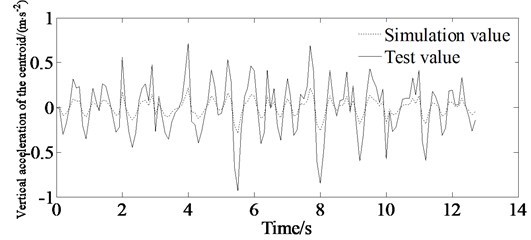
a) Vertical acceleration of the centroid

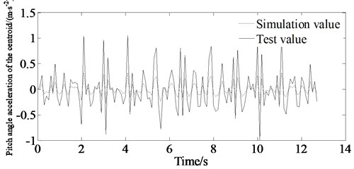
b) Pitch angle acceleration of the centroid

6. Conclusions

In this paper, the path tracking scenario is analyzed while the ADRC method is utilized for vehicle tracking the desired path. Accordingly, a 3-DOF simplified vehicle model and the tire model as well as the optimal preview time have been used to describe the motion by steering of the vehicle. Then the linear active disturbance rejection controller based on vehicle yaw rate is designed to solve the problem of path tracking maneuver.

To test the performance of the controller, simulation is operated and it is shown that the vehicle can track the prescribed path with the maximum absolute error of 0.11 m. Furthermore, the control method can be used to directly find an optimized trajectory. This is a main benefit of this method for path tracking control problem.

Comparison of the results of the ADRC method and the LQR method shows that the front steering angle based on the ADRC method is less than that of the LQR method, indicating that there is higher control effect for ADRC to solve the path tracking problem comparing with other traditional methods.

The pavement model in Carsim using C-class pavement data is established to simulate ride comfort. The correctness of the method is verified with a test vehicle. The result shows that it is practical to establish 3-D pavement and vehicle model to simulate ride comfort of vehicle in Carsim which can provide an effective method on the dynamic performance of vehicle for further research.

It is believed that the proposed control system can considerably improve vehicle handling and path tracking performance and provides valuable insight into the lane changes design work.

References

Wongun K., Dongwook K., Kyongsu Y. Development of a path-tracking control system based on model predictive control using infrastructure sensors. Vehicle System Dynamics, Vol. 50, Issue 6, 2012, p. 1001-1023.

Publisher
Funke J., Gerdes Christian J. Simple clothoid lane change trajectories for automated vehicles incorporating friction constraints. Journal of Dynamic Systems. Measurement and Control, Vol. 138, Issue 2, 2016, p. 1-9.

Publisher
Yang I. B., Na S. G., Heo H. Intelligent algorithm based on support vector data description for automotive collision avoidance system. International Journal of Automotive Technology, Vol. 18, Issue 1, 2017, p. 69-77.

Publisher
Rajaram V., Subramanian S. C. Design and hardware-in-loop implementation of collision avoidance algorithms for heavy commercial road vehicles. Vehicle System Dynamics, Vol. 54, Issue 7, 2016, p. 871-901.

Publisher
Lian Y., Zhao Y., Hu L., et al. Longitudinal collision avoidance control of electric vehicles based on a new safety distance model and constrained-regenerative-braking-strength-continuity braking force distribution strategy. IEEE Transactions on Vehicular Technology, Vol. 65, Issue 6, 2016, p. 4079-4094.

Publisher
Makoto I., Toshiyuki I. Design and evaluation of steering protection for avoiding collisions during a lane change. Ergonomic, Vol. 57, Issue 3, 2014, p. 361-373.

Publisher
Dang R., Wang J. Q., Li S. E., et al. Coordinated adaptive cruise control system with lane-change assistance. IEEE Transactions on Intelligent Transportation Systems, Vol. 16, Issue 5, 2015, p. 2373-2384.

Search CrossRef
Luo Y., Yong X., Kun C., Hiromitsu K. A dynamic automated lane change maneuver based on vehicle-to-vehicle communication. Transportation Research Part C Emerging Technologies, Vol. 62, 2016, p. 87-102.

Publisher
Esmaeil B., Ruey Long C., Sarkodie Gyan T. A binary decision model for discretionary lane changing move based on fuzzy inference system. Transportation Research Part C Emerging Technologies, Vol. 67, 2016, p. 47-61.

Publisher
Zachary S., Donald M., Sarkodie Gyan T. Reactive regulation of single-lane vehicle-road interactions. SAE Technical Paper, Vol. 1, Issue 390, 2014, p. 59-67.

Search CrossRef
Wu Mengxun, Deng Weiwen, Zhang Sumin, Sun Hao Modeling and simulation of intelligent driving with trajectory planning and tracking. SAE Technical Paper, Vol. 2, Issue 1, 2014, p. 59-67.

Search CrossRef
Miyake Hiroyuki An intuitive lane guidance function. SAE Technical Paper, 2016, https://doi.org/10.4271/2016-01-0080.

Publisher
Hou Yi, Edara Praveen, Sun Carlos Modeling mandatory lane changing using Bayes classifier and decision trees. IEEE Transactions on Intelligent Transportation Systems, Vol. 15, Issue 2, 2014, p. 647-655.

Publisher
Desiraju Divya, Chantem Thidapat, Heaslip Kevin Minimizing the disruption of traffic flow of automated vehicles during lane changes. IEEE Transactions on Intelligent Transportation Systems, Vol. 16, Issue 3, 2015, p. 1249-1258.

Publisher
Dang Ruina, Wang Jianqiang, Li Shengbo Eben, Li Keqiang Coordinated adaptive cruise control system with lane-change assistance. IEEE Transactions on Intelligent Transportation Systems Transactions on Intelligent Transportation Systems, Vol. 16, Issue 5, 2015, p. 2373-2383.

Publisher
Wang Qiushi, He Yuping A study on single lane-change manoeuvres for determining rearward amplification of multitrailer articulated heavy vehicles with active trailer steering systems. Vehicle System Dynamics, Vol. 54, Issues 1-102, 2016, p. 2016-123.

Publisher
Benloucif M. A., Popieul J. C., Sentouh C. Multi-level cooperation between the driver and an automated driving system during lane change maneuver. IEEE Intelligent Vehicles Symposium (IV) Gothenburg, Sweden, Vol. 19, Issue 22, 2016, p. 1224-1229.

Publisher
Guo Konghui, Ding Haitao, Zong Changfu Progress of the human-vehicle closed-loop system maneuverability’s evaluation and optimization. Chinese Journal of Mechanical Engineering, Vol. 39, Issue 10, 2003, p. 27-35.

Publisher
Zhang Lixia, Zhao Youqun, Wu Jie Research on vehicle handling inverse dynamics based on optimal control. China Mechanical Engineering, Vol. 18, Issue 6, 2007, p. 2009-2011.

Search CrossRef
Chen Zengqiang, Sun Mingwei, Yang Ruiguang On the stability of linear active disturbance rejection control on the stability of linear active disturbance rejection control. Acta Automatica Sinica, Vol. 39, Issue 5, 2013, p. 574-580.

Publisher

Cited by

Adaptive trajectory tracking control strategy of intelligent vehicle

(2020)

Driverless simulation of path tracking based on PID control

(2020)

About this article

Received

14 March 2017

Accepted

17 July 2017

Published

30 September 2017

SUBJECTS

Vibration in transportation engineering

DOI

https://doi.org/10.21595/jve.2017.18342

Keywords

vehicle handling dynamics

path tracking

ADRC

inverse problem

Acknowledgements

This paper was supported by the Science and Technology Program Foundation of Weifang under Grant 2015GX007 and the Foundation Research Funds for the Central Universities under Grant 3122016A004. The first author gratefully acknowledges the support agency.

This is an open access article distributed under the Creative Commons Attribution License, which permits unrestricted use, distribution, and reproduction in any medium, provided the original work is properly cited.

Previous article in issue Previous Next article in issue Next

Research article

2024 02 18

Optimal control of autonomous vehicle path tracking based on whale optimization algorithm

Fang Han, Yingjie Liu, Wen Peng

Research article

2023 08 01

Minimum-time lane changing problem of vehicle handling inverse dynamics based on adaptive mesh refinement and collocation optimization method

Yingjie Liu, Dawei Cui, Wen Peng

Research article

2022 08 17

Application of A* algorithm in intelligent vehicle path planning

Ruili Wang, Zhizhan Lu, Yunfeng Jin, Chao Liang

Research article

2017 09 30

Adaptive interval type-2 fuzzy logic systems for vehicle handling enhancement by new nonlinear model of variable geometry suspension system

Mansour Baghaeian, Ali Akbar Akbari

Y. Liu, D. Cui, and Y. Fu, “Path tracking control for inverse problem of vehicle handling dynamics,” Journal of Vibroengineering, Vol. 19, No. 6, pp. 4591–4608, Sep. 2017, https://doi.org/10.21595/jve.2017.18342

Copy Extrica

Copied to clipboard!

TY  - JOUR
DO  - 10.21595/jve.2017.18342
UR  - https://doi.org/10.21595/jve.2017.18342
TI  - Path tracking control for inverse problem of vehicle handling dynamics
T2  - Journal of Vibroengineering
AU  - Liu, Yingjie
AU  - Cui, Dawei
AU  - Fu, Yu
PY  - 2017
DA  - 2017/09/30
PB  - JVE International Ltd.
SP  - 4591-4608
IS  - 6
VL  - 19
SN  - 1392-8716
ER  - 

Copy Ris

Copied to clipboard!

@article{Liu_2017,
	doi = {10.21595/jve.2017.18342},
	url = {https://doi.org/10.21595/jve.2017.18342},
	year = 2017,
	month = {sep},
	publisher = {{JVE} International Ltd.},
	volume = {19},
	number = {6},
	pages = {4591--4608},
	author = {Yingjie Liu and Dawei Cui and Yu Fu},
	title = {Path tracking control for inverse problem of vehicle handling dynamics},
	journal = {Journal of Vibroengineering}
}

Copy Bibtex

Copied to clipboard!

[1]Y. Liu, D. Cui, and Y. Fu, “Path tracking control for inverse problem of vehicle handling dynamics,” Journal of Vibroengineering, vol. 19, no. 6, pp. 4591–4608, Sep. 2017, doi: 10.21595/jve.2017.18342.

Copy IEEE

Copied to clipboard!

Liu, Yingjie, Dawei Cui, and Yu Fu. “Path Tracking Control for Inverse Problem of Vehicle Handling Dynamics.” Journal of Vibroengineering 19, no. 6 (September 30, 2017): 4591–4608. https://doi.org/10.21595/jve.2017.18342.

Copy Chicago

Copied to clipboard!

Path tracking control for inverse problem of vehicle handling dynamics

Abstract

1. Introduction

2. Model of vehicle path tracking problem

2.1. Mathematical model of vehicle path tracking problem

2.2. Tire model

2.3. Optimal preview time

3. Design of linear active disturbance rejection controller based on vehicle yaw rate

4. Numerical simulation and experimental verification

4.1. Simulation result

4.2. Evaluation of calculation accuracy

4.3. Experimental result

4.3.1. Test objectives

4.3.2. Block diagram of test system and measurement equipment

4.3.3. Measurement equipment

4.3.4. Test procedure

4.4. Controller robustness verification in external disturbance environment

5. Rebuilding of road model and vehicle simulation of ride comfort based on Carsim

5.1. Road model

5.2. Vehicle model in Carsim

5.3. Simulation result

5.4. Experimental result

6. Conclusions

References

Cited by

About this article

Related Articles