Abstract
In order to reduce the time and space complexity of operational modal analysis (OMA) for slow linear time-varying (SLTV) structures based on moving window principal component analysis (MWPCA), this paper proposes a new moving window self-iteration principal component extraction (MWSIPCE) method. Different from getting principal components by singular value decomposition (SVD) or eigenvalue decomposition (EVD) in MWPCA algorithm, MWSIPCE just extracts the first-several-orders principal components by self-iteration. Comparing with MWPCA, MWSIPCE has lower time and space complexity. What’s more, this paper explains the reason of modal exchange in some data windows in detail, and gives an illustration to how to set window length . The OMA results on non-stationary vibration response simulation signal of time-varying cantilever beam under white noise excitation show that this method can well identify the time-varying transient modal parameters (natural frequencies and modal shapes) for SLTV structures and has less time and space consume, the algorithm is also more precise than MWPCA.
1. Introduction
Modal parameters (Natural frequencies, mode shapes) are essential for dynamics structural damage recognition, health monitoring [1] and independent modal space control [2]. From 1980s, operational modal analysis (OMA) deals with the estimation of modal parameters from vibration data obtained in operational rather than laboratory conditions [3]. OMA differs from experimental modal analysis (EMA) in that it seeks to determine a structure’s dynamic characteristics from response-only measurements, without precise knowledge of excitation forces. PCA is one of the most classic in multivariate analysis and data mining. The idea was first proposed by the Pearson in 1901, and it was used for the field of biology [4]. Principal components are linear combinations of the original data which help to visualize similarities in an ensemble of signals. Because all principal components are orthogonal and ordered according to the variance contribution of sample, the largest two or three principal components provide an excellent representation of variability within a set of data [5]. Traditional calculation method of PCA is using matrix decomposing, which includes SVD and EVD [6]. However, these ways calculate all principal components in one time, that makes the algorithm always has high time-space complexity. In 1969, NIPALS algorithm [7] is firstly proposed, different from traditional method, the algorithm iteratively calculates principal components. In order to reduce the time-space complexity of traditional PCA, this paper proposes a new self-iteration principal components extraction (SIPCE) algorithm which based on NIPALS algorithm.
With the development of science and technology, high speed, large, complicated and intelligent engineering structures in civil engineering field are applied more frequently. In working condition, these engineering structures usually need to experience a variety of harsh environments, which will lead to many engineering structures parameters (mass, stiffness and damping) changing over time inevitably. In practical engineering structures, the systems are often time-varying and the modal parameters are also changing with time, such as rockets in fight with mass lost [8], the trains crossing bridges [9], etc. YANG summarized the basic theory involved in modal parameter estimation of time-varying structures, including the introduction and discussion about the dynamic theory of linear time-varying systems that presented the dynamic model and the definition and properties of poles of linear time-varying systems. In addition, he established the criteria for slow time-varying systems in the time-domain and frequency-domain, providing the basis and assumptions for modal parameter estimation of time-varying structures respectively. Ramnath [10] pointed out the system whose variation in coefficient is much less than that in solution is called slow time-varying system.
In 1947, structure natural frequency and damping identification method were put forward by Kennedy and Pancu. After 70 years of development and progress, modal parameter identification has experienced from the linear time invariant (LTI) structures to slow linear time-varying (SLTV) structures. At present, OMA method learned from the latest research achievements in the field of control theory, system engineering and signal process [11], etc. Classical OMA method cannot apply to SLTV structures because of the non-stationary response data. The OMA methods of SLTV structures are based mainly on the assumption of short time invariant and “frozen” thought, which promoted modal analysis theory of LTI structures to SLTV structures, and identified the time-varying modal parameters. Another approach is using online or recursive technology to track the time-varying modal parameters [12]. Based on these theories, some popular methods were proposed, including time-frequency analysis based on wavelet transform (WT) [13, 14], Hilbert-Huang transform (HHT) [15], subspace methods [16], Auto Regressive Moving Average (ARMA) models [17], etc. However, these methods can only identify time-varying transient modal frequency of SLTV structures.
Guan et al. presented the method which combined principal component analysis (PCA) with moving window (MW) for operational modal parameters identification of SLTV structures [18]. That method is based on eigenvalue decomposition of PCA, so the complexity of time and space is very high. This study proposed a time-varying OMA method based on moving window self-iteration principal component analysis (MWSIPCE). MWSIPCE can well identify the time-varying transient modal parameters of SLTV structures and its time and space complexity is lower than MWPCA. Besides that, the reason of modal exchange in some data windows is explained, that has great engineering significance for fault monitoring.
2. OMA of LTI structures based on SIPCE
2.1. Mathematical model of PCA
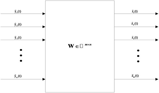
The data set of observation signals is composed by unrelated unknown latent variables through a linear transformation matrix , which is shown in Fq. (1) [19]:
Matrix meets condition:
Fig. 1 is the diagram of PCA model. The goal of PCA is to find linear transformation matrix and uncorrelated latent variables only from observed signal . The uncorrelated latent variables are called principal components of observation signal .
Fig. 1 is the diagram of PCA model. The goal of PCA is to find linear transformation matrix and uncorrelated latent variables only from observed signal . The uncorrelated latent variables are called principal components of observation signal .
Fig. 1Description of PCA problem
2.2. OMA of LTI structure based on PCA model
According to the theory of structural dynamics, for LTI structures with -degree-of -freedom, the equations of vibration motion in the physical coordinate is [18]:
In the Eq. (3): matrix is the mass matrix of the LTI structures, matrix is the damping matrix of the LTI structure, matrix is the stiffness matrix of the LTI structures, is the time. Matrix is the time domain random dynamic motivation of the LTI structures, and matrix is the time domain dynamic displacement response of the LTI structures, is the time domain dynamic speed response of the LTI structures. And is the time domain dynamic acceleration speed response of the LTI structures.
Viscous damping matrix can’t be orthogonally diagonalized by modal shape, so it can’t be decoupled directly. However, in special cases, matrix could be orthogonally diagonalized. For example, the viscous damping which is proposed by Rayleigh:
In Eq. (4), , denotes as the outside and inside damping constants of the system, for weak damping vibration system, the above model is effective.
For real modal analysis, in the modal coordinate, the random vibration response signals of mechanical structures with weak damping can be decomposed into the inner product of modal shapes and modal responses:
where is the output displacement, is the reversible modal shape matrix which composed by independent mode shapes , besides that, is basis-vector matrix in modal coordinate space and is the modal coordinate matrix which composed by modal response of each mode.
Plugging Eq. (5) into Eq. (3), which transports physical coordinate into modal coordinate:
Simplifying Eq. (6):
Then, Eq. (7) is the modal model, where is modal mass matrix, is modal damping matrix, is modal stiffness matrix:
Based on the vibration theory in Eqs. (5)-(13), when the structure’s natural frequencies of each mode are not equal, the modes vectors are orthogonal:
And modal response vectors are independent from each other. Then satisfies:
where is a real positive diagonal matrix.
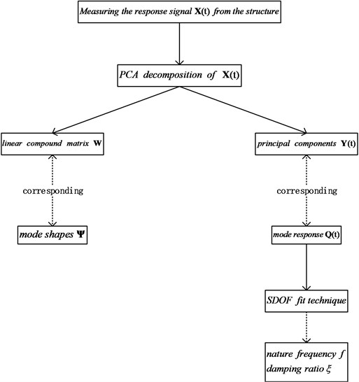
Natural frequency and damping ratio can be identified by FFT or single degree of freedom (SDOF) fitting techniques from mode coordinate response vector . Fig. 2 is the Schematic diagram of OMA based on PCA modal.
In view of Eq. (1) and Eq. (5), for random vibrations of weakly damped systems, there is a one-to-one mapping between the orthogonal mode matrix and the linear transformational matrix in Eq. (2). Besides that, there is a one-to-one mapping between modal response matrix in and the PCs . Therefore, the existence, uniqueness and deterministic of OMA based on PCA algorithm can be proved by PCA decomposition.
2.3. Self-iteration and principal component extraction algorithm
SIPCE algorithm is based on NIPALS algorithm. Firstly, choosing a column from the observation signal matrix . Then calculating the first principal component vectors and the first transformation matrix vector iteratively.
As Eq. (16) shows, updating error matrix to calculate the second principal component vectors and the second transformation matrix vector and so on:
Fig. 2Schematic diagram of OMA based on PCA modal
(1) Choosing the arbitrary column data vector, and assume that the chosen column is the th column. So, vector is got from signal matrix . denotes the th principal moment, and is the th loop which calculates the th principal moment, 1, 1, and ; Set the maximal number of iterations is .
(2) Calculate : ;
(3) Normalize the vector : ;
(4) Update : ;
(5) Compare the in the step (4) with the in the step (2). Define variable , and denotes accuracy requirement. If , their difference is in the prescribed scope (the algorithm is convergent). Then return to the step (6), or and return to the step (2).
(6) Calculate the error matrix:
(7) Calculate : .
(8) Define variable , is truncation error, if , and return to the step (1), calculate and .
The step (8) is to calculate the oversized contribution rates which correspond to the principal components. So, is the approximate contribution rate, which corresponds to the th principal component. Variable denotes cumulative variance proportion of the current principal component of calculated principal components.
Setting truncation error as . If , the current principal component is not important enough, the algorithm stops iteration, and the process of principal components extraction is end.
In the steps of the SIPCE algorithm, is the th principal component of the residual error matrix. The comparison of the in the step (5) is to judge whether meets the demand. If it does, the algorithm updates the error matrix and get the first principal component of the new error matrix . Eq. (17) and Eq. (18) show that the contribution of is larger than . In conclusion, is the first principal component of observation signal matrix, and is the second principal component and so on.
2.4. Approach of self-iteration and principal component extraction algorithm to OMA
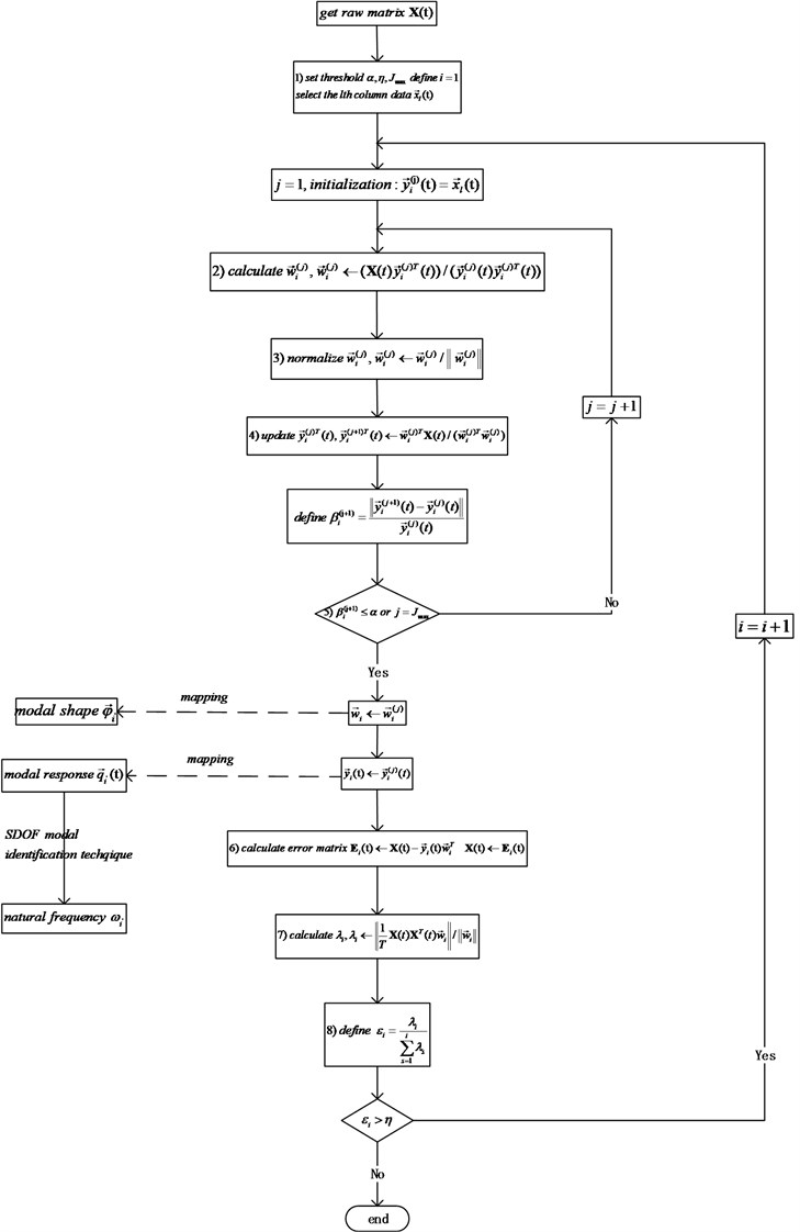
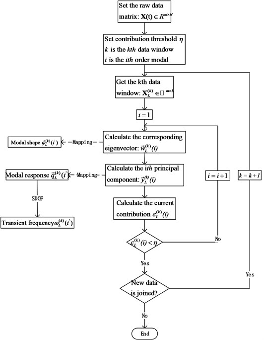
Fig. 3 shows the flow of OMA based on SIPCE. Variable represents the contribution of its corresponding principal components. denotes the importance measure of next principal components, and is a setting threshold value that we could use to control the iterations. Therefore, it realizes the principal components extraction.
2.5. The comparison between SIPCE and PCA
The traditional batch PCA gets linear transformation matrix and principal components by singular value decomposition (SVD) or eigenvalue decomposition (EVD) [20]. However, there are singular value and ill-posed problems in SVD and EVD [21, 22]. Because of these defects, the traditional batch PCA algorithm may not be able to accurately identify the modal vibration mode and natural frequency of the structures. SIPCE algorithm directly gets principal components by recursion, and the accuracy of self-iteration and principal component extraction results only depends on the threshold value. Therefore, self-iteration and principal component extraction based on OMA could avoid singular value decomposition of matrix and the ill-posed problems of eigenvalue decomposition effectively.
SIPCE calculates principal components one by one, and its goal is to identify several order models by user requirements. However, traditional batch principal component analysis gets all principal components by matrix decomposition. That not only increases the computation time, but also spends lots of memory to store large matrices.
3. OMA of SLTV structures based on MWSIPCE
3.1. OMA of SLTV structures based on “Time-freezing” theory
Based on the assumption of “time-invariant” in a minor interval, the countless SLTV structures sets could be gotten by mass, stiffness and damping matrix of each instantaneous moment in “freezing” time-varying. The set is expressed by Eq. (19):
Equation is the LTI structures at moment, and the set of is “time-freezing” represent of SLTV structure . Because the SLTV structures and LTI structures have the same mass, stiffness and damping matrixes at every moment, the varying characteristics of them are equipotent [23, 24].
For small damping structures, the collected data of the structure response can be divided into several parts. And in the th part (data window), the modal coordinates can decompose the response of the linear structure:
Fig. 3The flowchart of OMA based on self-iteration principal component extraction algorithm
The variables and are modal shape matrix and modal response vector of the th data window. We normalize main orthogonal modal shape vector to meet each modal response that is independent when each structure natural frequency are unequal. Then the natural frequency can be identified from modal respond as well as OMA of LTI structure are based on PCA:
3.2. OMA of SLTV structure based on MWSIPCE
3.2.1. The model of MWSIPCE
In order to identify time-varying transient modal parameters, we divide a time quantum into many minimum transient and then identify the modal parameters of every transient by the SIPCE. The process of segmentation can be mathematically modeled as Fig. 4 shows, and rectangular window is selected to add new data and discard part of old data. Variate is to express the th data window .
Fig. 4The rectangular data window with moving window length L
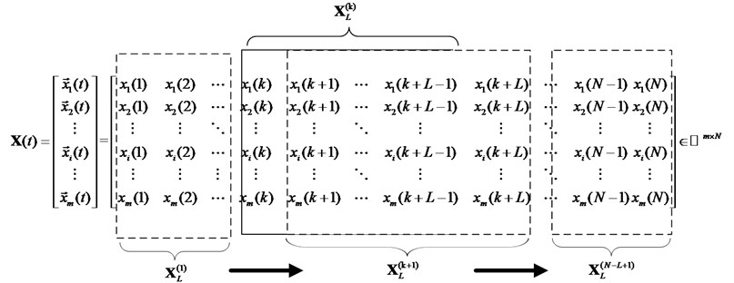
Setting the raw data matrix with variables and samples when the rectangular data window with memory length is introduced, and then the raw data matrix will be changed into . With sampling length, is used to estimate the statistical average modal value of middle time. When the transient time is changed, the rectangular window moves. In addition, the data window matrix will be updated as Fig. 4 shows. Therefore, the transient mathematical model of time-varying structure is built, and then combines every transient to identify SLTV structure modal parameter.
Based on the assumption of short time invariant and “frozen” thought, at every transient time, the structure is regarded as a LTI structure. Then, identifying the modal parameters in every rectangular data window by SIPCE. The OMA of SLTV structures is turned into the OMA based on SIPCE for LTI structures. In the end, we combine the modal of every transient by curve-fitting technique, then measure and monitor the modal parameters of SLTV structures real-timely.
Fig. 5 shows the flow of MWSIPCE. For the raw matrix , the algorithm gets the transient data window , and then calculate the principal components and the corresponding change vector. Updating the data window until all transient modal parameters are calculated.
Fig. 5The flowchart of OMA based on MWSIPCE for SLTV
3.2.2. The selection of window length
As an important parameter for MWSIPCE based Operational Modal Identification under a slow SLTV Structure, the window length should not be too large or too small. If the window length is too long, the non-stationary random response signals of the slow SLTV structure cannot approximately be seen as the stationary random response of LTI structure. The th order statistical average mode nature frequency and statistical average modal shapes during periods are not regarded as an approximate evaluations of transient mode nature frequency , and transient mode shapes at time. If the window length is too short, identification error will be larger owing to inadequate sample and large frequency resolution. Moreover, the precision of identified natural frequencies got by FFT depends on frequency resolution . It is more precise when the length of FFT is larger. And is inversely proportional to sampling frequency . Frequency resolution of FFT is defined [25]:
The factors effect the choice of window length is showed below:
1) The changing speed of SLTV structure and non-stationary degree of vibration response signal. If the SLTV structure is fast changed, there is a high non-stationary degree and we should reduce the window length . Define average frequency variation of the th mode in a data window as :
where variables , , , are end-frequency of the th mode, begin frequency of the th mode, end-time, begin-time of the whole data.
2) Sample frequency of vibration response signal and frequency resolution . Window length is proportional to sample frequency and frequency resolution .
3) The power of storage and computing for embedded structure. The memory and computation of MWPCA and MWSIPCE mode are proportional to moving window length [26]. Furthermore, computation of FFT is depending on window length .
3.3. The comparison between MWSIPCE and MWPCA
In order to ensure the precision of time-varying transient modal parameter identification based on assumption of short time invariant, the response time should be divided into minimum period, so that we could produce many response data.
According to user requirements, comparing with MWPCA algorithm calculates all components in each rectangular data window, MWSIPCE algorithm just extracts several principal components in each rectangular data window and does not need to calculate other components. Therefor MWSIPCE algorithm mostly reduces time complexity. Besides that, MWSIPCE iteratively gets principal parameters, so, it doesn’t need to store many large matrixes and avoids the ill-posed or singular value problems.
For raw data , different algorithms are compared in various aspects. The size of space complexity depends on whether the program stores past matrixes. And the results are expressed in Table 1.
MWSIPCE algorithm is more precise than MWPCA algorithm. Moreover, it enhances the efficiency of operating modal parameter identification.
Table 1The comparison of algorithm performance
Algorithm | Time complexity | The least space complexity | Algorithm robustness |
MWPCA based on EVD | High | Ill-posed problems | |
MWPCA based on SVD | High | Singular value problem | |
MWSIPCE | Low | Avoids the ill-posed and singular value problems |
3.4. The reason of modal exchange in MWSIPCE
Based on MWSIPCE algorithm, the frequencies of SLTV structure are ordered by the contribution rather than the frequency value. At one transient, the contributions of each identified modal can be represented as , and they meet the following relationship:
For SLTV structure, engineering structure parameters (mass, stiffness and damping) change over time, so the modal contribution rate of each order is time-varying. Therefore, there is a special phenomenon called modal exchange. Therefore, contribution order is not equal to the frequency order, the correspondence of two ranking order maybe change over time. For example, at transient time , there is a one-to-one match between the first-four-order identified modal and the first-four-order real modal, but at transient time , the third order identified modal is corresponded to the forth-order real modal and the forth-order identified modal is corresponded to the third-order real modal.
For SLTV structure, MWSIPCE algorithm can find modal exchange based on changing frequency, and monitor running state of SLTV structure. CPV denotes project require, at moments, is the variance contribution of the first 3 order PCs. With the new data is added, the contribution of the third modal is decreasing and the forth order’s contribution is increasing. Maybe at a moment , when the CPV meets project requirement, the modals involved in CPV are the first order, the second modal and the forth modal.
3.5. Limitations and applications of time-varying OMA based on moving-window MWSIPCE
Time-varying operational modal analysis with MWSIPCE method has the following limitations and application scores:
1) Each order of modal shapes gotten by PCA is normalized orthogonal, which loses amplitude information. This is a characteristic of PCA or ICA based OMA and a characteristic of MWSIPCE based time-varying OMA.
2) It can just apply to slow linear time-varying structures. Only for slow linear time-varying structures, the theory of “time-freezing” is established, and the non-stationary random response signals of the slow LTV structures can approximately be seen as the stationary random response time series of LTI structures in short time interval.
3) The length of moving window is selected with prior knowledge of time-varying speed of LTV structure and fixed. However, the length of moving window . should be fully self-adaptive selected and changed only by nonstationary vibration response signals when there is no prior knowledge of time-varying speed then.
4) PCA method for operational modal analysis can identify mode shapes, modal frequencies and mode damping ratios for LTI structure only from stationary vibration response signals. MWSIPCE method for operational modal analysis can also identify time-varying transient mode shapes, modal frequencies and mode damping ratios only from non-stationary vibration response signals. However, theoretical analysis and numerical simulation indicate that mass decreasing or moving will generates an additional damping [27, 28] for LTV structure. So, the time-varying transient mode damping ratio identified by LMRPCA method cannot be compared with mode damping ratio calculate by FEM directly.
5) The modes which calculated by SIPCE are ordered by the contribution of vibration response rather than frequency. For time-varying structure, the contribution of each mode is varying. MWSIPCE is based on SIPCE, there might be modal exchange in the calculation.
4. Simulation verification of time-varying transient operational modal identification
In order to validate the accuracy and efficiency of MWSIPCE method, we set up a dynamic model of a time-varying cantilever beam, and analysis the influence of mass change for time-varying structure. A simulation with cantilever beam is designed, which is a time-varying structure whose mass is changing over time. For experimental verification, additional damping caused by moving mass and the limitation of experimental condition make it quite difficult [29], so simulation verification is a frequently used method. In the generation of simulation data, we gave full consideration to boundary conditions, and the Gaussian noise is added into the data to simulate real scene. The algorithm can be well validated by the simulation of time-varying cantilever beam [25].
4.1. Evaluation criteria
Theoretical values and FEA values are set as standard, which are calculated under the condition of undamped real modal shape and undamped real modal nature frequency, and MWPCA algorithm is based on EVD method.
In order to quantitatively compare the modal vibration mode, modal assurance criterion (MAC) is investigated [30], which is an important standard when considering the effectiveness of modal shape identification [31]. Eq. (25) is the detailed equation of calculated MAC value:
where is the identified shape, represents the real shape, and () represents the inner product of the two vectors. MAC values oscillate between 0 (no coincidence) and 1 (complete coincidence), The more MAC value is close to 1, the more accurate estimated shape is. However, MAC just can reveal the information of direction and shape, the size of amplitude-mode is not contained.
4.2. Parameters of time-varying cantilever beam
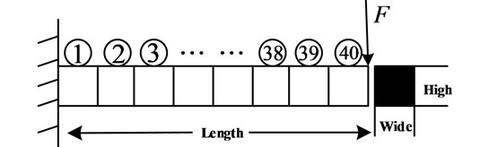
The dimension of cantilever beam model is 1 m×0.02 m×0.002 m (length×height×width) while cross sectional area 410-4 m2, density 7860 kg/m3, moment of inertial , and 3×10¹¹ N/m2 is Young’s modulus. Time-varying mass property is simulated by changing the density of beam, given as Eq. (26):
The simulation time is set as 4 s, and the first ten order time-varying natural frequency values at the start and finish time are compared in Table 2.
Table 2The change curve of natural frequencies (0-4 s)
t/s | Order | |||||||||
1 | 2 | 3 | 4 | 5 | 6 | 7 | 8 | 9 | 10 | |
0 s | 16.9997 | 104.6552 | 293.038 | 574.2391 | 949.2649 | 1418.0561 | 1980.635 | 2637.0355 | 3384.3056 | 4231.5200 |
4 s | 19.6807 | 123.3374 | 345.3485 | 676.7473 | 1118.71 | 1671.1952 | 2334.2016 | 3107.7761 | 3991.9779 | 4986.8942 |
In Finite element method (FEM), the continuum cantilever beam is generally dispersed with finite multi-degree-of-freedom structures and the mass, stiffness and damping matrices can be expressed as follows:
where , and are time-varying element mass, stiffness and damping matrices respectively. denotes proportional damping matrix, and is the length of each element. And are the proportional coefficients with responding to mass and stiffness matrices, respectively.
In FEM, the continuums beam is divided into 40 elements, each finite element is an output. Only one translational freedom and one rotational freedom are considered for each node without axial freedom, which is depicted in Fig. 6.
The forced response signals are acquired by Newmark – . The proportional coefficients are set as 4×10⁻⁴, and 1×10⁻⁷. The initial velocities and displacement are zero while the white noise is imposed as excitation. From Table 2, it is found that the frequencies are increasing over time. As frequency is 4986.8942 Hz at the finish time, the sampling frequency is set as 10000 Hz based on sampling theorem. The simulation time is set as 4 s while integration step is 1/10000 s for Newmark-, and the number of sample points 40000.
Level of 2.0 % Gauss measurement noise is added into response signals in time domain. The calculation formula of noise is as follows:
In Eq. (30), denotes a normal random vector, its mean value is zero and standard deviation is one. is the noise level. The measurement noise level above is 2.0 %.
Fig. 6FEM Model of cantilever beam
4.3. Parameters of time-varying OMA based on MWSIPCE
1) Limited memory length is set as 4096 data points [25].
2) Set precision threshold 0.000001.
3) Set maximum number of iteration 100.
4) Set truncation error 0.05.
5) Computer configuration
Operating system: 64-bit Windows 10.
Manufacturer: HP.
System Type: HP Z240 SFF Workstation.
Processor: Intel(R) Core(TM) i5-6500 CPU @ 3.20GHz (4 CPUs).
Memory: 8192MB RAM.
Programing language and environment: MATLAB 2014a.
4.4. Time-varying transient modal parameters identification results
In the FFT figure, the FFT peak frequency (horizontal axis) is corresponding to the nature frequency. Fig. 7(a-d) shows the first three order nature frequencies that identified by MWSIPCE at random moments (0.9954 second, 1.4954 second, 2.4954 second, 3.4954 second).
Fig. 8(a-d) shows the first three order shapes that identified by MWSIPCE at random moments, and the modal shapes are normalized (The moments are same as Fig. 7).
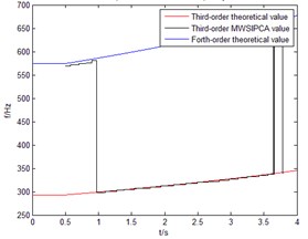
Connecting the nature frequency at every moment Comparison results of the first three orders frequency between theoretical calculation and MWSIPCE are shown in Fig. 9. The frequency identification changes from 0.5 second to 3.7048 second.
Fig. 10 is the records of the MAC values at every moment, and we have corrected the correspondence when there is modal exchange in the third order. The frequency identification changes from 0.7048 s to 3.7048 s, and we just identify the absolute time-varying transients to ensure recognition accuracy. The calculated equation is showed in section 4.1.
For MWSIPCE algorithm, its accuracy depends on threshold . Table 3 is the precise MAC comparison of the third order between MWPCA and MWSIPCE at some moments. Table 4 is the self-MAC of some moments to check the modal vector orthogonality.
Table 5 is the comparisons of time-space consumptions. MWSIPCE extracts the first 4 order modes, which meet the requirement.
Fig. 7FFT of the first three orders principal components at random moments
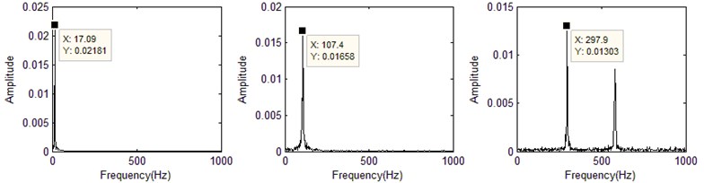
a) 0.9954 second
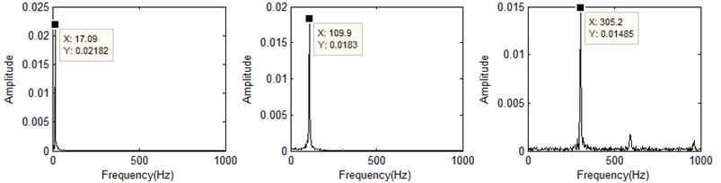
b) 1.4954 second
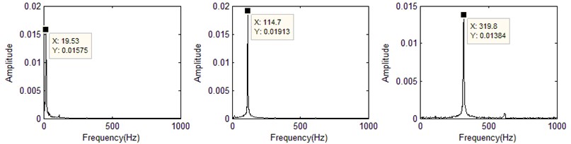
c) 2.4954 second
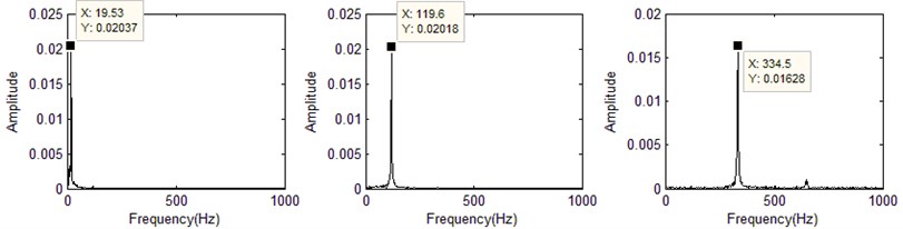
d) 3.4954 second
Table 3Comparison of MAC the third order between MWPCA and MWSIPCE at some moments
Moments (s) | MWPCA | MWSIPCE |
1.3153 | 0.7580 | 0.8607 |
1.3336 | 0.6878 | 0.8125 |
1.3763 | 0.5679 | 0.7068 |
1.4612 | 0.6740 | 0.8212 |
Fig. 8Modal shape comparison between MWSIPCE and theoretical value
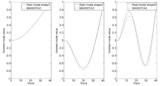
a) 0.9954 second
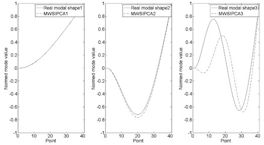
b) 1.4954 second
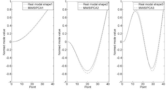
c) 2.4954 second
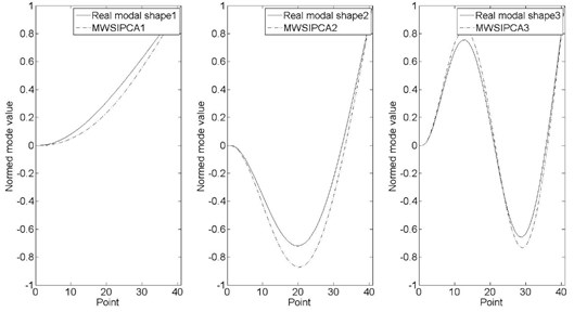
d) 3.4954 second
Fig. 9The frequency comparison of cantilever beam
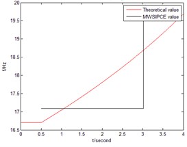
a) The first order
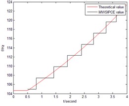
b) The second order
c) The third order
Fig. 10MAC value of every moment
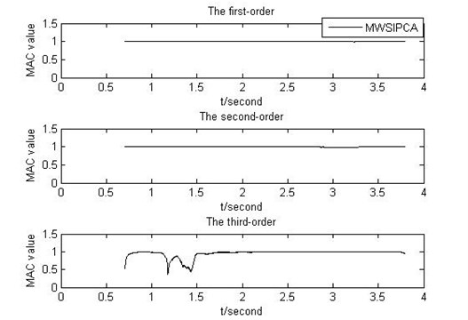
Table 4The self-MAC of some moments
1.0201 s | 2.0201 s | 3.0201 s | |||||||||
Order | 1 | 2 | 3 | Order | 1 | 2 | 3 | Order | 1 | 2 | 3 |
1 | 1.000 | 0 | 0 | 1 | 1.000 | 0 | 0 | 1 | 1.000 | 0 | 0 |
2 | 0 | 1.000 | 0 | 2 | 0 | 1.000 | 0 | 2 | 0 | 1.000 | 0 |
3 | 0 | 0 | 1.000 | 3 | 0 | 0 | 1.000 | 3 | 0 | 0 | 1.000 |
Table 5Time-space consumptions based on MWSIPCA
Method | Absolute time consumption (s) | Memory consumption (MB) |
MWPCA | 374.135 | 7196 |
MWSIPCE | 200.397 | 2397 |
4.5. The analysis of simulation results
When the time is in the interval of 0.5002 s-0.972 s and 3.6520 s-3.7820 s, there is a big deviation between the third-order frequency identified by MWSIPCE and the third-order theoretical value. However, the third-order frequency identified by MWSIPCE is similar to the forth-order theoretical value. In addition, it is because in these transient times, the contribution rates of the third modal and the forth modal are changed, so the third modal identified by MWSIPCE is changed. As we can see in Table 2, the third-order modal frequency identified by MWSIPCE is corresponding to the forth-order nature frequency. Because of the modal exchange, Fig. 8(c) shows that the third-order real shape is corresponding to the fourth-order modal shape, which is identified by MWSIPCE.
Fig. 7, Fig. 8, Fig. 9 and Fig. 10 approve that MWSIPCE algorithm can identify the modal shape and nature frequency of SLTV structure accurately. Table 3 shows that MWSIPCE is more precise than MWPCA at some moments. The reason is there are singular value decomposition of matrix or the ill-posed problems for MWPCA. Table 4 shows that the different modal shapes identified by MWSIPCE are complete orthogonal.
When the limited memory length is 8192, 1.22 Hz is less than 12.2436 Hz and the identified effect is good while it needs high time and space complexity. When the limited memory length is 2048, its 4.88 Hz is more than 3.0609 Hz. In addition, it needs low time and space complexity, but the identified effect is the worst, even in some time, the modal parameters are not identified for the data points are not enough. Therefore, the limited memory length is chosen to be 4096 according to compromise, because its 2.44 Hz is less than 6.1218 Hz and its time and space complexity is not too high.
MWSIPCE algorithm extracts several principal components from every rectangular data window. The number of identified order depends on the requirements of the user. However, MWPCA must calculate all components. Table 5 shows that the MWSIPCE algorithm has less time and space consumption.
5. Conclusions
The simulation results of cantilever beam show that the MWSIPCE method can track the time-varying transient modal frequency and modal shape of SLTV structure well. Simulation results show that MWSIPCE needs less time and space consumption than MWPCA, and it real-timely measures and monitor SLTV structure. Furthermore, this paper gives detail explanations to the modal exchange in the simulation, which has great significance for malfunction monitoring of SLTV structure. Besides, the article illustrates the way of setting length and the limitation of MWSIPCE method.
However, this study has some limitations. Each order of modal shapes got by PCA is normalized orthogonal, which loses amplitude information. It may be inappropriate to use average values to estimate the intermediate time for a period of time in the FFT of PCs, which would cause more burrs in the results of FFT of PCs. In the simulation verification, level of 2.0 % Gauss measurement noise is added into response signals to simulate the noise in the real scene, the design of real experiments and experimental verification of SIPCE are the future work. The next research is to identify the modal parameters in real-time using on-line and recursive techniques and integrate the algorithms into embedded device for mechanical fault diagnosis. How to select scientifically and adaptively is also a future study.
References
-
Rainieri C., Fabbrocino G., Manfredi et al. G. Robust output-only modal identification and monitoring of buildings in the presence of dynamic interactions for rapid post-earthquake emergency management. Engineering Structures, Vol. 34, 2012, p. 436-446.
-
Cinquemani S., Resta F. A mechanical approach to the design of independent modal space control for vibration suppression. Journal of Vibration, Acoustics, Stress, and Reliability in Design – Transactions of the ASME, 135, p. 2013-51002.
-
Reynders E. System identification methods for (operational) modal analysis: Review and comparison. Archives of Computational Methods in Engineering, Vol. 19, 2012, p. 51-124.
-
Pearson K. On lines and planes of closest fit to systems of points in space. Philosophical Magazine, Vol. 2, 1901, p. 559-572.
-
Trbovic N., Dancea F., Langer T., Günther U. Using wavelet de-noised spectra in NMR screening. Journal of Magnetic Resonance, Vol. 173, 2005, p. 280-287.
-
Lei B., Soon Y., Tan E. L. Robust SVD-based audio watermarking scheme with differential evolution optimization. IEEE Transactions on Audio, Speech, and Language Processing, Vol. 21, Issue 11, 2013, p. 2368-2378.
-
Wold H., Lyttkens E. Nonlinear Iterative Partial Least Squares (NIPALS) Estimation Procedures. Bulletin of the International Statistical Institute, Vol. 43, 1969.
-
Lei Li The Modal Analysis of Industrial Application in the Incident of the Spacecraft Structure. Fudan University, 2011.
-
Marchesiello S., Bedaoui S., Garibaldi L., et al. Time-dependent identification of a bridge-like structure with crossing loads. Mechanical Systems and Signal Processing, Vol. 23, Issue 6, 2009, p. 2019-2028.
-
Ramnath R. V. Multiple Scales Theroy and Aerospace Application. Reston, Virginia, AIAA, 2010.
-
Spiridonakos M. D., Poulimenos A. G., Fassois S. D. Output-only identification and dynamic analysis of time-varying mechanical structures under random excitation: A comparative assessment of parametric methods. Journal of Sound and Vibration, Vol. 329, Issue 7, 2010, p. 768-785.
-
Klepka A., Uhl T. Identification of modal parameters of non-stationary systems with the use of wavelet based adaptive filtering. Mechanical Systems and Signal Processing, Vol. 47, Issues 1-2, 2014, p. 21-34.
-
Ghanem R., Romeo F. A wavelet-based approach for the identification of slowly linear time-varying dynamical systems. Journal of Sound and Vibration, Vol. 234, Issue 4, 2000, p. 555-576.
-
Zhiyu Shi, Lin Shen Parameter identification of slowly linear time-varying dynamics system based on wavelet method. Journal of Vibration, Measurement and Diagnosis, Vol. 28, Issue 2, 2008, p. 108-112.
-
Roveri N., Carcaterra A. Damage detection in structures under traveling loads by Hilbert-Huang transform. Mechanical Systems and Signal Processing, Vol. 28, 2012, p. 128-141.
-
Tasker F., Bosse A., Fisher S. Real-time modal parameter estimation using subspace methods: Theory. Mechanical Systems and Signal Processing, Vol. 12, Issue 6, 1998, p. 797-808.
-
Larbi N., Lardies J. Experimental modal analysis of a structure excited by a random force. Mechanical Systems and Signal Processing, Vol. 14, 2000, p. 181-192.
-
Wei Guan, Cheng Wang, Liang Xiang, Chen D. S. OMA following moving window PCA for slowly linear time-varying multi-degree-of-freedom system. Journal of Information and Computational Science, Vol. 12, Issue 7, 2015, p. 2779-2793.
-
Wang C., Guan W., Gou J., et al. Principal component analysis based three-dimensional operational modal analysis. International Journal of Applied Electromagnetics and Mechanics, Vol. 45, Issues 1-4, 2014, p. 137-144.
-
Abdi H., Williams L. J. Principal component analysis. Wiley Interdisciplinary Reviews: Computational Statistics, Vol. 2, Issue 4, 2010, p. 433-459.
-
Mishra A. K., Motaung T. Application of linear and nonlinear PCA to SAR ATR. 25th International Conference on Radioelektronika (Radioelektronika), Bratislava, Slovakia, 2015.
-
Wall M. E., Rechtsteiner A., Rocha L. M. Singular Value Decomposition and Principal Component Analysis. A Practical Approach to Microarray Data Analysis. Springer, US, 2003, p. 91-109.
-
Kaiping Yu, Shiwei Pang, Jie Zhao Time-varying linear/nonlinear structural parameter identification and system identification method. Chinese Science Bulletin, Vol. 20, 2009, p. 3147-3156.
-
Petsounis K. A., Fassois S. D. Non-stationary functional series tarma vibration modelling and analysis in a planar manipulator. Journal of Sound and Vibration, Vol. 231, Issue 5, 2000, p. 1355-1376.
-
Wang C., Wang J., Zhang T. Operational modal analysis for slow linear time-varying structures based on moving window second order blind identification. Signal Processing, Vol. 133, 2017, p. 169-186.
-
Jiang Z. J., He X. B., Yang Y. P. Adaptive time-varying process monitoring basing on fast MWPCA. Journal of Nanchang University (Natural Science), Vol. 32, 2008, p. 198-204.
-
Chicheng M. A., Xinong Zhang, Yajun Luo, Chunlin Zhang Dynamic analysis on a fluid-structure coupling system with variable mass in a rectangular tank. Journal of Xi’an Jiaotong University, Vol. 48, Issue 7, 2014, p. 109-116.
-
Chicheng M. A., Xinong Zhang, Yajun Luo, Shuai Zhang Dynamic responses for a fluid-structure coupling system with variable mass in a tank of spacecraft. Journal of Aerospace Engineering, Vol. 30, Issue 3, 2015, p. 736-745.
-
Zajaczkowski J., Lipiński J. Instability of the motion of a beam of periodically varying length. Journal of Sound and Vibration, Vol. 63, Issue 1, 1979, p. 9-18.
-
Zhou S. D., Heylen W., Sas P., et al. Parametric modal identification of time-varying structures and the validation approach of modal parameters. Mechanical Systems and Signal Processing, Vol. 47, Issue 1, 2014, p. 94-119.
-
Junqing Bai, Guirong Yang, Cheng Wang Modal identification method following locally linear embedding. Journal of Xi’an Jiaotong University, Vol. 47, Issue 1, 2013, p. 85-89.
Cited by
About this article

This work was financially supported by National Natural Science Foundation of China (Grant No. 51305142, 51305143), China Postdoctoral Science Foundation Project (No. 2014M552429), Postgraduate Scientific Research Innovation Ability Training Plan Funding Projects of Huaqiao University (No. 1511314011).
Tianshu Zhang implemented the method and completed the experimental verification. He also writhed the paper. Cheng Wang proposed the ideas, and gave guides in writing the paper. Jianying Wang provided with the data, and helped accomplish the experiment. Yewang Chen gave help in algorithm optimization. Yiwen Zhang helped modify English mistakes.
