Abstract
Numerical simulation of a novel fuzzy control and back propagation neural network (BPNN) control for divergent instability based on classical flutter of 5-DOF wind turbine blade section driven by pitch adjustment has been investigated. The work is dedicated to solving destructive flap/lag/twist divergent instability from classical flutter, which might occur during the gust wind action, and might cause fracture failure of the blade itself and tower body. In order to investigate the optimal control method, the parameters of blade section are specially designed so as to simulate the actual situation, which lead to absolutely divergent motions (ADM) under gust wind load. The control of ADM often leads to limit cycle oscillation (LCO), the larger amplitude of which is likely to cause fracture failure of tower body. A novel fuzzy control method with adjustable quantization gain and BPNN control strategy are investigated in order to effectively eliminate LCO (leading to direct convergence of the system) or reduce the amplitude of LCO. The obvious effects of fuzzy control and BPNN control are illustrated by numerical comparisons of vibration suppression from nonlinear time response, amplitude of LCO and frequency spectrum analysis. An experimental platform is built based on hardware-in-the-loop simulation by way of PLC-OPC technology in order to test the real-time performance of the control algorithm. The feasibility of the control algorithm is demonstrated by the experimental results displayed by touch-screen hardware.
1. Introduction
The flutter instability of wind turbine blades usually includes two cases: classical flutter instability and stall flutter instability. Although stall flutter instability has generally been an important issue in flutter research recent years, classical flutter was observed involving a high-speed rotating blade under gust load. Especially under extreme conditions, divergent instability issues of classical flutter may become a more important design consideration. For example, in September 2013, the typhoon event in Shanwei (China) [1], the maximum instantaneous wind speed reached 62.5 m/s, which resulted in not only flap/lag failure (from stall flutter instability) of a large number of wind turbine blades, but also fracture failure (from divergent instability of classical flutter) of the tower body.
Most of the literature of classical flutter focused on the helicopter blades, or non-coupling wing sections [2, 3]. However, the classical flutter studies of wind turbine blades are still rare. The aeroelastic stability of a three-bladed wind turbine was considered with respect to classical flutter for a MW sized turbine, with critical frequency computed [4]. Don W. Lobitz discussed the classical flutter issue in an infinite aerofoil undergoing oscillatory pitching and plunging motion in an incompressible flow based on Theodorsen’s technique [5]. Baran R. P. gave a literature study on classical flutter and obtained theoretical background information on BLADEMODE V.2.0 and PHATAS [6]. The influence of the large deformation on the performance was introduced and the classical flutter instability was investigated in literature [7]. Flutter instability was discussed both in frequency and time domains in terms of blade tip flap/lag/twist deformations [7]. Classical flutter and active control of single-cell thin-walled composite wind turbine blade beam based on piezoelectric actuation with small deformation and constant wind loads were analyzed [8]. However, all these literatures were based on either Theodorsen’s technique which has been modified over the years in a variety of ways to simplify the solution procedure, or computations using the time-domain ADAMS/AERODYN software. Moreover, most of them are based on constant wind load. How to effectively realize classical flutter control for a large blade with pitch motion and variable wind load has become an important research needed to be investigated.
The divergent instability might be produced by vertical loads which make the system conservative. The instability type involving the cracked beam depends on the crack flexibility parameter, the boundary conditions as well as the non-conservativeness parameter [9]. In present study, in order to maximize the control performance and investigate the optimal control method for divergent instability, the sectional parameters are specially designed with ADM [10], i.e. even if the wind speed is small, the system is still in an unstable state of divergent instability. Classical flutter for the purposes of LCO analysis is defined as the coupling of the bending and torsional modes, which is rarely observed. While flow separation is not necessary for this type of flutter, structural and fluidic non-linearities are present in the experiment as a stable LCO was achieved in reference [11]. In present study, when the specific frequency ratio and damping ratio are designed for ADM, the LCO vibration in control process can also be observed. However, the conventional PID controller has lost its usefulness here. A novel fuzzy PID control based on maximum error tracking method with adjustable quantization gain is investigated to realize flutter suppression for classical flutter with ADM so as to avoid fracture failure of the tower body to the utmost. For the purpose of comparison, BPNN PID control for divergent instability from classical flutter based on pitch adjustment is also investigated. Meanwhile in this area, the investigation of typical 2D blade section based on flap/lag or flag/twist motion plays an important role due to its simplicity and high efficiency; so, in this study, researches on aeroelastic instability and flutter control will be depicted based on a 5-DOF blade section. Both fuzzy PID and BPNN PID can produce LCO vibration. Whereas amplitudes and spectra are usually used to analyze LCO vibration [12], the role of initial parameters in the formation of LCO and different control methods based on analysis of response amplitude and frequency structure are discussed.
In addition, real-time effects of control algorithms (for the independent airfoil cross-section) are investigated by an experimental platform based on hardware-in-the-loop simulation by way of PLC-OPC technology, which provides a kind of operation method and platform based on laboratory conditions for the real-time control of virtual objects. The implementation process of PLC-OPC communication technology can be described as follows: the aeroelastic system model is run in MATLAB/SIMULINK environment; the controlled output of the aeroelastic model is directly entered into the corresponding PLC memory via SIMULINK's “OPC Write” module; the control algorithm is run entirely in PLC system; and the driving signal sent by PLC is output to the aeroelastic model via “OPC Read” module.
2. Analytical model
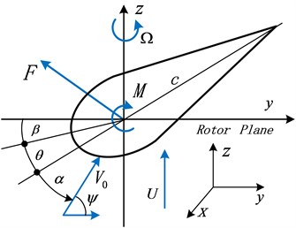
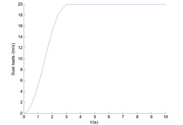
The 5-DOF blade section structure is designed in such a way that its motions have five independent translational degrees of freedom: an edgewise direction (lag), denoted ; one perpendicular to that (flap), denoted ; another twisted angle, denoted ; variable pitch angle , and rotating angle (see Fig. 1(a)). The classical aerodynamic forces are denoted by lift and moment . The wind velocity is denoted by , with relative wind angle denoted by In order to simulate the extreme state, present study uses a kind of gust wind load, as shown in Fig. 1(b).
In order to maximize the control performance, the sectional parameters listed in Table 1 are specially designed with ADM, while the wind speed 4 m/s, the three system movements are still divergent.
It is assumed that the distance between the centre of gravity and the elastic axis is small enough, at the same time regardless of the impact of the masses determining the sum of inertia of the rotor, gearbox and generator. Based on analysis of Lagrange’s equations, the blade tip sectional flap/lag/twist motions are respectively described as [13]:
Fig. 1a) Coordinate system and b) gust load
a)
b)
Table 1The blade sectional parameters
Iterms | Values | Iterms | Values |
Natural frequency | 6 rad s-1 | Damping ratio | 0.02 |
Natural frequency | 8 rad s-1 | Damping ratio | 0.08 |
Natural frequency | 4 rad s-1 | Damping ratio | 0.02 |
Mass per length | 15 kg m-1 | 1/4 chord length by | /4 |
Rotational inertia | 10 mkg | Blade length | 20 m |
Length of chord (at ) | 0.3 m | Tip speed ratio | 1.2 |
Distance between center of gravity and center of elasticity /6 | |||
The classical linear models including piston theory and full potential flow models are widely used in aeroelastic design for their advantage of computational efficiency [14]. The aerodynamic model is used here in order to quickly investigate a wide range of initial parameters that control the behavior of the nonlinear system in Eq. (1). Since the classical flutter problem refers to the linear flow regime, a linear aerodynamic theory was deemed sufficient. The linear aerodynamics of lift and moment can be approximatively expressed as [15]:
where is the air density; the inflow wind speed is expressed as:
3. Pitch adjustment based on intelligent control
Most of pitch control processes for wind turbine are realized by intelligent control strategy. A hybrid controller based on PI and fuzzy technique for the pitch angle controller was analyzed in order to improve power quality and maintain the stable output from wind farm [16]. A nonlinear control i.e. integral sliding mode control was proposed to regulate rated power at above rated wind speed by pitch control [17]. Two types of artificial neural network controllers including multi-layer perceptions with back propagation learning algorithm and radial basis function network were used to investigate the influences of pitch control [18]. However almost all these similar papers today focus on power control and conversion, wind energy utilization, and multivariable and nonlinear control so as to achieve maximum performance. Present study mainly focuses on the flutter control of divergent instability rather than power control. Meanwhile for the sake of comparison, two control methods, fuzzy PID control and BPNN PID control, are applied in this study.
3.1. Pitch actuator
Pitch adjustments of most large wind turbines today are realized by a series of hydraulic pitch actuators. Reference [19] used a hydraulic pitch actuator, which is a crank swing block using a kinematic scheme of blade rotation mechanism to realize pitch control. In view of this hydraulic system is a six-order system, and in order to make the pitch motion of the section closer to the actual situation, it is reasonable to find a new model for sectional unit system, with fewer states such that the input/output behaviour is changed as little as possible. Based on the six-order transfer function system in reference [19], the Optimal Hankel norm [20-21] is used here to make model reduction, with the states corresponding to the smallest Hankel singular values discarded. Hence a new model with two-order transfer function structure suitable for section unit can be obtained. Furthermore, applying the Laplace Inverse Transform for this two-order transfer function structure, the pitch actuation behavior can be described by two-order differential equation model as:
where is the pitch angle requested by the actual hardware controller.
Fig. 2 illustrates the effectiveness of model reduction characterized by the unit step responses. The unit step response after model reduction of Eq. (3) is very close to the result without model reduction in reference [19]. Meanwhile after the reduction, the curve is smoother with better stability.
Fig. 2The response of model reduction in present study vs. that without model reduction in reference [19]
![The response of model reduction in present study vs. that without model reduction in reference [19]](https://static-01.extrica.com/articles/18240/18240-img3.jpg)
3.2. Fuzzy PID control strategy
The requested pitch angle can be implemented by PID controller using the rotating speed error :
where , and are proportional gain, integral gain and derivative gain, respectively; and is a given initial rotating speed determined by initial wind speed .
It should be noted that most of the pitch control strategies in the previous literatures are based on linear control after linearization process [13]. The present control is the direct control of the nonlinear system, and of more practical significance.
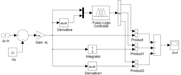
Parameters , and can be tuned to optimize control performance by control strategy. Fuzzy control depends on the fuzzy algorithm between the information of process and control input. Fuzzy controllers from their inception have demonstrated a vast range of applicability to processes where the control actions can be described in terms of linguistic variables, and can be used to improve the performance of a nonlinear system. For this rotating speed feedback system, fuzzy PID controller is devised in Fig. 3, with fuzzy rules developed based on Sugeno type. Two input variables, error of (E) and change in error (ED), and three output variables , and with seven linguistic variables of membership functions are used. The input linguistic variables are NB (Negative big), NM (Negative medium), NS (Negative small), ZE (Zero), PS (Positive small), PM (Positive medium) and PB (Positive big), respectively. Seven gbell--membership function forms for both E and ED (), are determined the same, which are shown in Fig.4. Borders of both function sequences vary between ±0.3. There are 49 weight values in PID parameter design. According to intuition method, lists of linguistic rules are shown in Tables 2-4.
It should be stated that according to the intuition method, the determination of fuzzy rules is a complex process, with operating experience playing a decisive role. Also, Eq. (1) is actually a nonlinear system, with different initial values determining quite different time responses. Therefore, for these gusty responses under different initial wind values, it is difficult to uniformly determine the ranges of error, scaling factors and other parameters. In particular for different initial wind values, it is a complex process to simultaneously adjust the membership function range in Fig. 4 and the PID parameter values in Tables 2-4. Here a novel maximum error tracking method for the determination of fuzzy rule is demonstrated as follows:
1) Preliminary determine the maximum speed () error range between ±0.3.
2) According to intuition method [20], the values of the Mamdani forms of the rules of the PID parameters (take for example) are determined as:
If E = NB, and ED = NB, NM, NS, ZE, PS, PM, and PB, respectively, then PB(), PB(), PM(), PM(), PS(), ZE(), and ZE(), respectively, which correspond to the first row values in Table 1.
Fig. 3The structure of fuzzy PID controller
3) Let the values of the Sugeno forms of the rules of the PID parameters (still take for example) directly change according to the magnitude of the maximum speed error. It is depicted as:
NB(), NM() /6×4, NS()/6×2, ZE() = 0, PS()/6×2, PM()/6×4, PB(). Hence rewrite the values of the Mamdani forms of the rules of as:
0.3, 0.3, 0.2, 0.2, 0.1, 0, and 0, respectively, which are exactly equal to the first row values in Table 1. Other fuzzy rules can be determined similarly.
4) A special quantization gain is designed in Fig. 3, which can be manually adjusted to a reasonable range to meet the requirements of the scaling factors for all different initial wind speeds (within 0 m/s-20 m/s). Appropriate range of quantization gain in present study is between 10-3-10-5. Furthermore, the values of beyond this range will make the control fundamentally ineffective, or bring about the occurrence of unexpected deviations, which is precisely the subtlety of this design.
Fig. 4Membership function plots
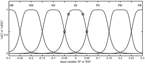
Table 2Rules for Kp
E\ED | NB | NM | NS | ZE | PS | PM | PB |
NB | 0.3 | 0.3 | 0.2 | 0.2 | 0.1 | 0 | 0 |
NM | 0.3 | 0.3 | 0.2 | 0.1 | 0.1 | 0 | 0 |
NS | 0.2 | 0.2 | 0.2 | 0.2 | 0 | –0.1 | –0.1 |
ZE | 0.2 | 0.2 | 0.1 | 0 | –0.1 | –0.1 | –0.2 |
PS | 0.1 | 0.1 | 0 | –0.1 | –0.1 | –0.2 | –0.2 |
PM | 0.1 | 0 | –0.1 | –0.2 | –0.2 | –0.2 | –0.3 |
PB | 0 | 0 | –0.2 | –0.2 | –0.2 | –0.3 | –0.3 |
Table 3Rules for Ki
E\ED | NB | NM | NS | ZE | PS | PM | PB |
NB | –0.3 | –0.3 | –0.2 | –0.2 | –0.1 | 0 | 0 |
NM | –0.3 | –0.3 | –0.2 | –0.1 | –0.1 | 0 | 0 |
NS | –0.3 | –0.2 | –0.1 | –0.1 | 0 | 0.1 | 0.1 |
ZE | –0.2 | –0.2 | –0.1 | 0 | 0.1 | 0.2 | 0.2 |
PS | –0.2 | –0.1 | 0 | 0.1 | 0.1 | 0.2 | 0.3 |
PM | 0 | 0 | 0.1 | 0.1 | 0.2 | 0.3 | 0.3 |
PB | 0 | 0 | 0.1 | 0.2 | 0.2 | 0.3 | 0.3 |
Table 4Rules for Kd
E\ED | NB | NM | NS | ZE | PS | PM | PB |
NB | 0.1 | –0.1 | –0.3 | –0.3 | –0.3 | –0.2 | –0.1 |
NM | 0.1 | –0.1 | –0.3 | –0.3 | –0.3 | –0.2 | –0.1 |
NS | 0 | –0.1 | –0.2 | –0.2 | –0.1 | –0.1 | 0 |
ZE | 0 | –0.1 | –0.1 | –0.1 | –0.1 | –0.1 | 0 |
PS | 0 | 0 | 0 | 0 | 0 | 0 | 0 |
PM | 0.3 | –0.1 | 0.1 | 0.1 | 0.1 | 0.1 | 0.3 |
PB | 0.3 | 0.2 | 0.2 | 0.2 | 0.1 | 0.1 | 0.3 |
3.3. BPNN PID control strategy
In view of the empirical fuzzy rules and regulative method of fuzzy control, at the same time, in view of the superiority of neural network control itself, and in order to compare with the fuzzy control, another method of BPNN control with back propagation learning algorithm [22] is investigated in this study.
BPNN is a perceptron network in which each neuron is connected with a number of input arcs. It is associated with each neuron having weight , which represents a factor to a value passing to the neuron. The BPNN PID control strategy uses an adaptive training algorithm based on a gradient descent approach to update network weights and ensures that the designed neural network is able to calculate the desired PID parameters. The incremental digital PID control algorithm can be expressed as:
Generally, the artificial neural network connects independent and decided variables through the neurons of input layer, hidden layers and transmit output layer. The present design is a four-input-three-output BPNN with three layers: input layer, one single hidden layer and output layer.
Four inputs of BPNN are:
Output of each neuron in the input layer is expressed as:
Input/output pair of each neuron in the hidden layer is expressed as follows:
where is the number of neurons in the hidden layer. is the symmetrical activation function (log-Sigmoid function) [20].
Input and output signals of each neuron in the output layer are:
where is the non-negative activation function (log-Sigmoid function) [20]. Hence the learning algorithm of the weight update (according to gradient descent algorithm) in output layer can be expressed as:
and the learning algorithm of the weight update in hidden layer is expressed as:
where 0.25 is learning rate, 0.05 is momentum factor, and , are:
4. Results and discussions
Considering the three equations of motions in Eqs. (1) and the pitch actuation expression in Eq. (3), and inserting Eq. (4) coupled with corresponding fuzzy structure or BPNN structure, and assuming:
result in the equations governing the whole nonlinear aeroelastic system as follows:
where , and all are nonlinear matrix variables described in Appendix, with their matrix variable elements comprised of: , , , , , , and wind speed .
Eq. (15) can be solved by nonlinear time integration scheme with nonlinear residual analysis by an internal iterative procedure in reference [23]. In the solution process, since the coefficient matrix is not a square matrix, the inverse operation of the matrix requires pseudo inverse operation. Aeroelastic instability analysis and control can be implemented by time responses, analysis of phase plane and limit cycle, and frequency spectrum analysis. Influences of different initial wind velocities and comparisons of two different control methods are demonstrated. The obvious effects of flutter suppression for divergent instability cases are displayed.
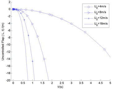
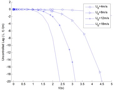
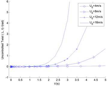
Fig. 5The uncontrolled blade tip responses of flap/lag/twist motions for different cases under different initial wind speeds
4.1. Divergent instability cases
The discrete gust can be used singly or in multiples to assess blade response to large wind disturbances. The mathematical representation of the discrete gust can be found in reference [24], with the gust amplitude and the gust length displayed in Fig. 1(b).
Fig. 5 shows the uncontrolled blade tip responses of flap/lag/twist motions for different cases under different initial wind speeds 4, 8, 12, and 18 m/s (all within the range of gust load), respectively. As depicted in aforementioned ADM state, all the three motions are in states of rapid divergences. Especially for flap/lag motions of 8, 12, and 18 m/s, all the displacements are rapidly divergent, and more than the blade length of 20 m within the 5 s time. This is precisely the ADM phenomenon mentioned above: assuming that the blade is long enough, over time, the magnitudes of all the divergent displacements will be incredible, even for smaller initial wind speeds (for example 4 m/s). According to the experience of ADM displacement control, it is difficult to achieve the states of complete convergences for all the divergent motions. Hence the follow-up study for divergent instability control will often present the limit cycle vibration state. Some cases intended to highlight the effects of two control methods under conditions of 8, 12, and 18 m/s are presented below, with time response analysis and LCO vibration demonstrated.
All the responses diverge rapidly in a matter of seconds, which means that the period is infinite and the magnitude is also infinite. It should be stated that in cybernetics, it is an extremely divergent unstable system, which is exactly what the author describes as the ADM system.
4.2. Influences of fuzzy control on divergent instability
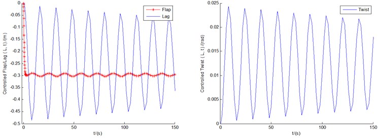
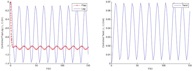
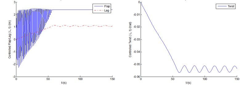
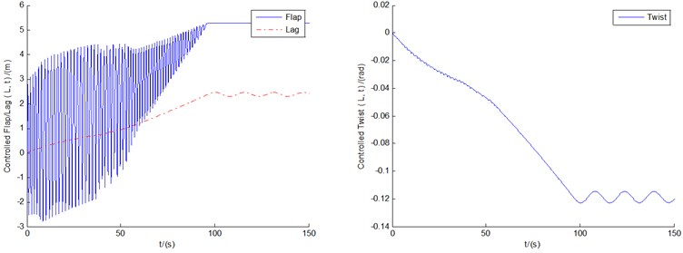
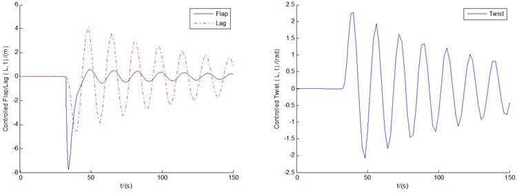
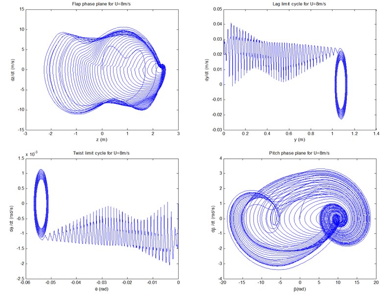
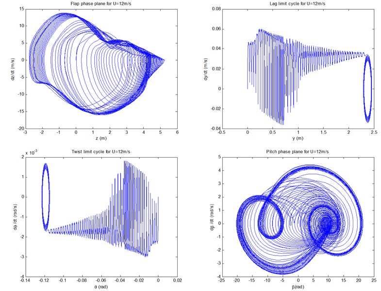
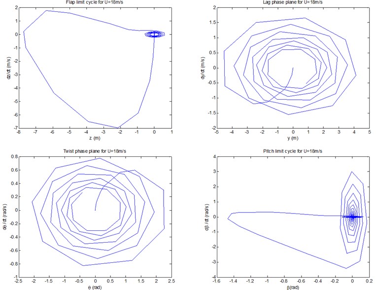
Fig. 6 show the controlled responses of the three motions and pitch motion by fuzzy controller under conditions of 8, 12, and 18 m/s, respectively. It can be seen that the controlled flap/lag/twist displacements and the pitch motion all show convergent or equal amplitude states, with the very small amplitudes of vibrations displayed. In other words, in contrast with uncontrolled cases, the controlled displacements are of more advantages from the viewpoint of amplitude suppression. It can also be demonstrated that all the three controlled flap motions, and the lag/twist motions in 18 m/s, are likely to show the states of LCOs as time goes on.
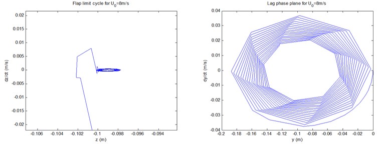
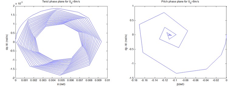
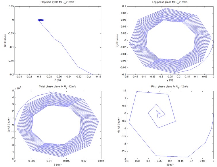
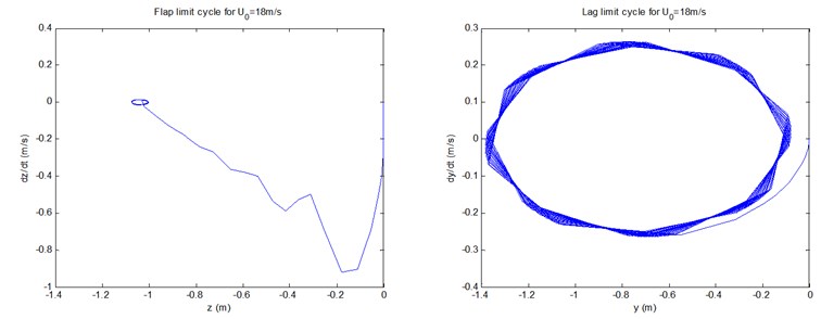
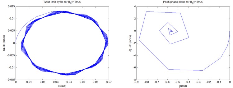
Fig. 7 show the controlled phase planes of the three displacements and pitch motion by fuzzy controller under conditions of 8, 12, and 18 m/s, respectively. It can be demonstrated that all the three controlled flap displacements, and the lag/twist displacements in 18 m/s, do show the states of the limit cycle vibrations. In particular, the scopes of amplitudes of the limit cycles of the three flap displacements are 0.002×0.002, 0.001×0.0067, and 0.07×0.0267, respectively, which demonstrate apparent aeroelastic control effect on divergent instability. In addition, all the starting points of the limit cycles and the phase planes are point (0, 0). The other phase planes in Fig. 7 will converge to fixed points as time goes on, the stability sates of which coincide with those demonstrated in Fig. 6.
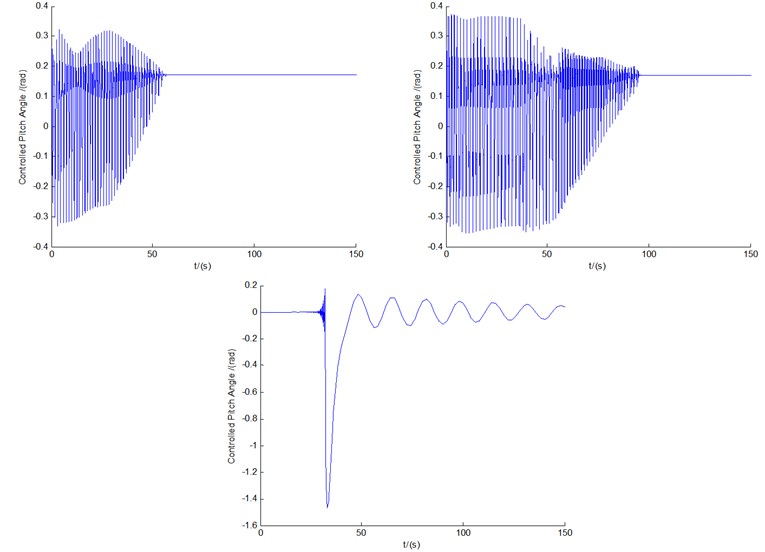
Fig. 6The controlled responses of the three motions and pitch motion by fuzzy controller under conditions of U0= 8, 12, and 18 m/s, respectively
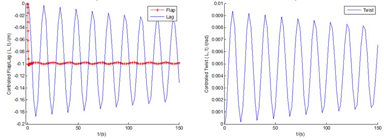
a)8 m/s
b)12 m/s
c)18 m/s
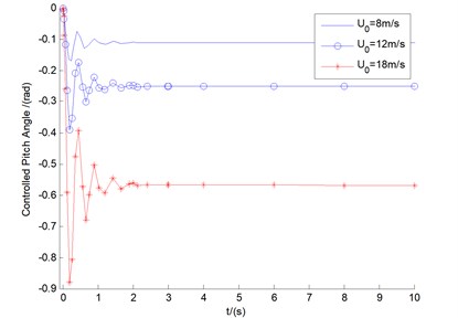
d) The controlled pitch angles in 8, 12, and 18 m/s, respectively
Fig. 7The controlled phase planes and LCOs of the three displacements and pitch motion by fuzzy controller under conditions of U0= 8, 12, and 18 m/s, respectively
a)8 m/s
b)12 m/s
c)18 m/s
4.3. Influences of BPNN control on divergent instability
Fig. 9(a)-(c) show the controlled responses of the three motions and pitch motion by BPNN controller under conditions of 8 m/s and 12 m/s, respectively. Also, the controlled flap/lag/twist displacements and the pitch motion all show convergent or equal amplitude states as time goes on. In contrast with the corresponding controlled cases in Fig. 6, vibration amplitudes of the BPNN control are slightly larger, but still within the ideal range of control. At the same time, the latter is also accompanied by a larger pitch power consumption. The additional difference between the fuzzy control cases and the BPNN cases is that the controlled lag/twist displacements of the BPNN cases might show the states of LCOs as time goes on, while the flap motions tend to converge stably.
Fig. 8The controlled responses of the three motions and pitch motion by BPNN controller under conditions of U0= 8, 12, and 18 m/s, respectively
a)8 m/s
b)12 m/s
c)18 m/s
d) The controlled pitch angles in 8, 12, and 18 m/s, respectively
Fig. 9(a)-(b) show the controlled phase planes and LCOs of the three displacements and pitch motion by BPNN controller under conditions of 8 m/s and 12 m/s, respectively. All the controlled lag/twist displacements do show the states of the limit cycle vibrations. All the flap phase planes will converge to fixed points as time goes on, convergent characteristics of which are in qualitative agreement with those from corresponding time responses in Fig. 8.
Anyway, above numerical simulations show an expected conclusion, namely that for flutter suppression of divergent instability, fuzzy control (based on maximum error tracking method and quantization gain) and BPNN control, each can play an important role in enhancing the vibration behavior of the classical flutter. Moreover, the former is more accurate, but it requires more complex experience. On the contrary, the latter does not require operational experience, but requires a higher level of programmable technology. In addition, for blade with ADM sate, no matter for what kind of control method, the generation of LCOs cannot be avoided, so the amplitudes control of limit cycle vibrations is very important.
Fig. 9The controlled phase planes and LCOs of the three displacements and pitch motion by BPNN controller under conditions of U0= 8, 12, and 18 m/s, respectively.
a)8 m/s
b)12 m/s
c)18 m/s
4.4. Vibration periods of LCOs
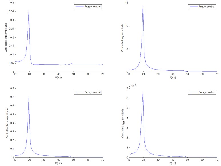
The vibration period (including period of LCO) is another indicator of vibration performance, which is usually reflected by the frequency structure from Fast Fourier Transformation(FFT) analysis. Take the case of initial 12 m/s; for example, Fig. 10 shows the frequency distribution diagrams of both fuzzy control(a) and BPNN control(b) under 12 m/s. Fequency structures of different iterms including flap/lag/twist motions and the requested pitch angle are demonstrated. From Fig. 10(a) we can see that the first frequencies of flap/lag/twist motions and the requested pitch angle all are within scope of 18-20 Hz, which are much smaller than the other corresponding ones (within the scope of 1050-1200 Hz) in Fig. 10(b). This means that the vibration periods of different terms of fuzzy control are much larger than those of BPNN control, which indicates the greatly improved flutter stability. Of course, this does not mean that the greater the vibration cycle, the better the performance, because too large a cycle means divergence. The same is true for the second frequencies: the second frequencies within range of 48-50 Hz in Fig. 10(a) are far less than those within range of 1150-1340 Hz in Fig. 10(b).
This can also be confirmed not only from the change trends of time responses in Fig. 6(b), but also from the phase planes and LCOs in Fig. 7(b). It also can be seen that the frequency distribution diagrams of flap motion and the requested pitch angle Fig.10(b) have large fluctuations, which means the relatively low stability and higher control consumption. This can also be confirmed from the time responses in Fig. 8(b).
In addition, take the controlled flap amplitude in Fig. 10(b) of BPNN control with 12 m/s, for example. The spectrum processing process can be summarized as follows. In the simulation solution, the variable step size method is used. Since the data points are very large and the frequency coverage range is 103Hz-3×10⁵Hz, furthermore the frequencies are symmetrical about 1.5×10⁵Hz. In present study, only half of the spectrum is taken to avoid the laborious time-consuming process. At the same time, it can effectively reduce the influence of frequency aliasing of the two parts of the left and the right. Furthermore, the meaningful spectrum region is 103 Hz-2×10³ Hz. Especially the ‘big’ spectrum at 1×10³ Hz is exactly the main lobe of the spectrum in the sinc form which is from truncated window function in time domain and should be filtered out. Thus, in this study, the frequency of display coordinates starts with 1050 Hz. Hence, Fig. 10(b) shows exactly what the analysis needs.
There are also a few points that need to be explained as follows: the unit of the amplitude in Fig. 10 is the result of normal FFT processing. However, the amplitudes of the BPNN controller cases are much higher than the fuzzy PID ones. Take the controlled flap amplitude in Fig. 10(b) of BPNN control with 12 m/s, for example. The response of the controlled flap displacement has a lot of frequency aliasing within 90s. This creates a great deal of overlap of amplitude. Although the frequency domain can also be expanded, the time at which the peak corresponds does not change. Therefore, in present study, frequency spectrum analysis is concerned only with frequency location structure, without regard to amplitude results. Another reason is that in the spectrum analysis, there is still the problem of truncation in time domain. This is equivalent to multiplying a rectangular weighting function. Compared with the fuzzy control, BPNN control in itself with more weighted signals, hence the frequency amplitude will be affected by more sinc function signals. Of course, none of this affects the expression of frequency structure in abscissa axis.
As for the frequency structure of uncontrolled system in Fig. 5, the same treatment can be implemented. However, it is meaningless to display the spectrum of the uncontrolled signal. This is because the truncation time of the time domain in Fig. 5 is very short 5 seconds as mentioned above, which means that a very small rectangular window function is loaded. Therefore, in the frequency domain, a sinc function of wide width will be convolution, which seriously affects the spectrum of the original signal. Of course, some tests tried to increase the time of signals in Fig. 5, say, for 300 seconds. The results that the numerical solution time was too long, and the amplitude was too large to infinity, and even the simulation would be terminated, which is exactly what the ADM system indicates.
In addition, it should be stated that the steady-state value of the PID parameter is not necessarily fixed at a single value. Fig. 11 demonstrates the change of the coefficients of PID controller of both fuzzy control(a) and BPNN control(b) under 12 m/s, respectively. As time goes on, all the parameters can be stabilized. However, parameter of BPNN controller is either equal to 0 over time, or equal to 1. In addition, the parameter frequencies of initial fluctuations within 45 s-100 s of BPNN controller are greater than those of Fuzzy controller, which demonstrates the relatively complex regulation performance of BPNN controller, on the other hand, the initial stage adjustment of BPNN controller is also easy to cause frequency aliasing. Another point to note is that the conventional PID controller has lost its usefulness here, even the widely used optimal PID controller based on ITAE optimization criteria can, the conventional fuzzy control algorithms, and the conventional neural network algorithms [25] not be done here, which is exactly the reason why the new intelligent control methods are developed for ADM blade in present study.
5. Real-time effects of control algorithms
Because the large wind power system is mostly controlled by PLC, the design of the controller adopts the SIEMENS S7-200 controller in present study. Due to the possibility of singular values in the simulation process, or the possibility that the numerical value of the control is too large, in the real-time control of the process, there might be a hardware interrupt or downtime. Or because the sampling time is too small, and the controller computation is too large, there will be a memory overflow problem. Therefore, the validity of the control algorithm needs to be verified in real-time operation.
Fig. 10Frequency structures of responses of both a) fuzzy control and b) BPNN control under U0= 12 m/s, respectively
a)
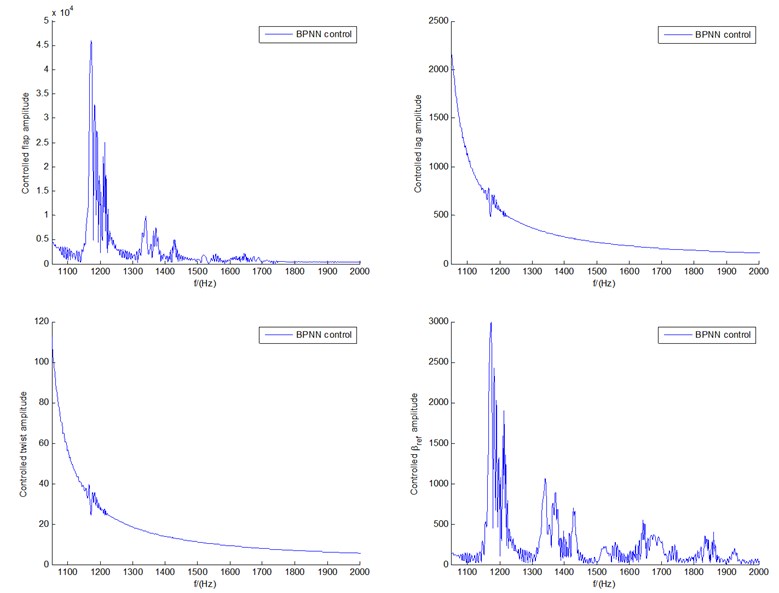
b)
Fig. 11The change of the coefficients of PID controller of both a) fuzzy control and b) BPNN control under U0= 12 m/s, respectively
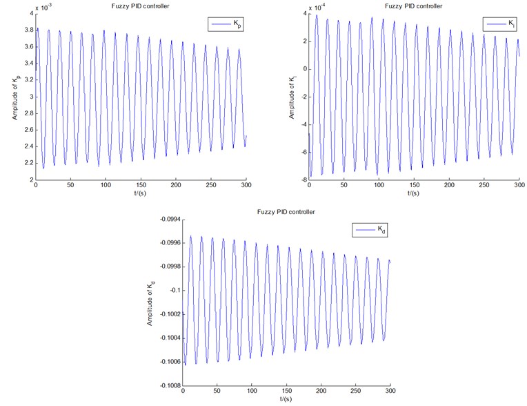
a)
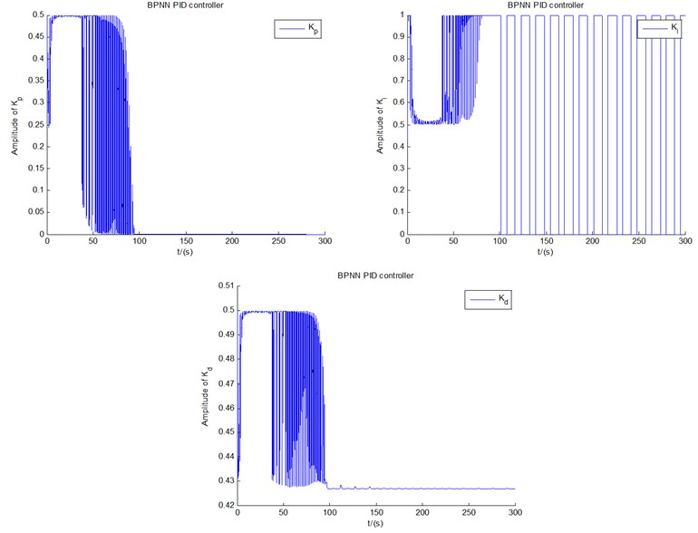
b)
For example, the controller system in Fig. 12(c) contains two modules of CPU 224XP. If a single CPU module is used, memory overflow errors may occur during the BPNN operation. However, for fuzzy control process, a single CPU module is sufficient. Of course, the sampling time should not be too small. The platform can detect in actual control, which control algorithm is more easily implemented in the project, and which control is more security, but also has a control system cost performance problem. Hence in view of the processor speed of the controller hardware, memory limitations, and possible hidden singularity during parameter simulation, the real-time effects of the two control methods should be tested. An experimental platform is built in present study to investigate the real-time effects of control algorithms. Due to testing and control of the independent airfoil(section) cannot be carried out under laboratory conditions, also in light of the effectiveness of MATLAB/SIMULINK in simulation of complex system, the experimental platform is built based on hardware-in-the-loop simulation by way of PLC-OPC technology [26] in Fig. 12. The OPC Read/Write blocks read/write data from/into PLC by items on OPC server. Fuzzy or BPNN control is fully implemented in PLC controller. Touch screen HMI is connected to the “port0” port of PLC, which can display the displacement signals, the pitch adjustment signal and the PID parameter process signals, etc.
Fig. 12The experimental platform built by PLC-OPC technology
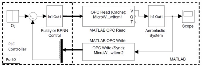
a) The experimental platform scheme
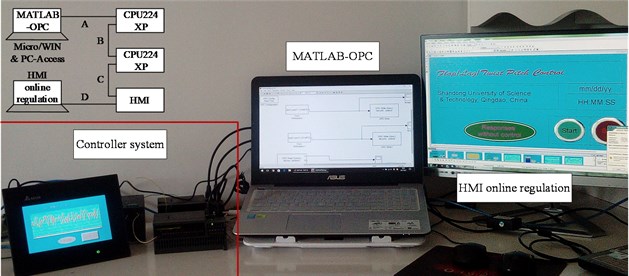
b) The photograph of the platform
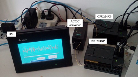
c) Controller system
In addition, the values and curves of other displacements, as well as the process curve of pitch adjustment, can also be displayed in the HMI interface. It should be noted that the implementation of technical route of PLC-OPC technology, as well as settings and adjustments of the communication parameter (including data types, sampling frequency and sampling points, etc.) is a complex process. Especially the data structure and variable type defined in the connection links, must be consistent with each other in storage performance. In order to ensure the appropriate accuracy and moderate computing time, the characteristics of communication parameters comprise a number of features such as: OPC Write mode is synchronous, with sample time being 0.1 s; OPC Read mode is from cache, with sample time between 0.1 s-1 s, and with value data type being single type; the data address defined in OPC server is the type of double word corresponding to S7-200 PLC memory, with data type being real type; the data type defined in HMI system is float, with sample time being 1 s.
Fig. 13Real-time effects of fuzzy control and BPNN control displayed in HMI
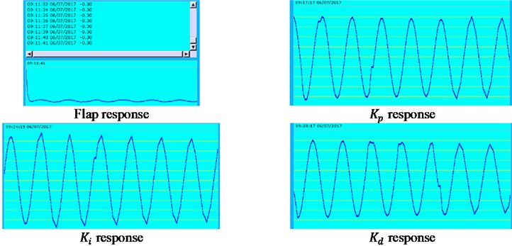
a) Real-time effects of fuzzy contol
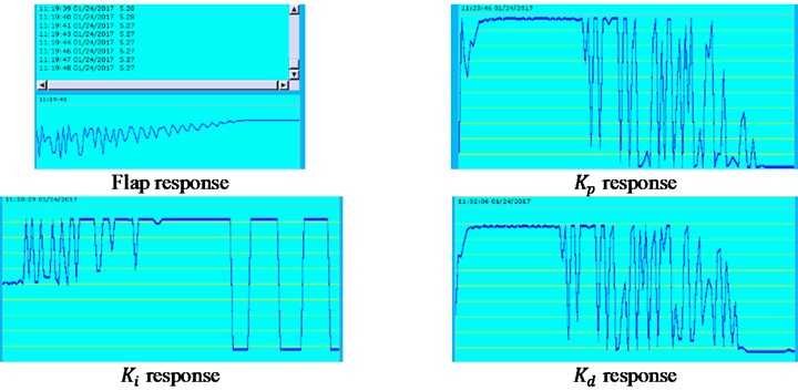
b) Real-time effects of BPNN control
Still take the previous case under initial 12 m/s; for example, real-time effects of fuzzy control(a) and BPNN control(b) are displayed in HMI in Fig. 13. Two flap responses in Fig. 13 reproduces the values and graph curves of flap displacements in Fig. 6(b) and Fig. 8(b), respectively, which shows considerable consistency. Notice that in Fig. 13(a), the value of the flap scrolling bar is –0.3, which is consistent with the steady value shown in the graph in Fig. 6(b). Responses of PID parameters , , and in Fig. 13 show the adjustment and fluctuation of the PID parameters in both fuzzy PID control and BPNN PID control process in Fig. 11. Take BPNN control as an example, and are finally stable near zero and at 0.4271, respectively, while is either equal to 0 over time, or equal to 1. Furthermore, binarization of (0 or 1) may be the cause of the limit cycle vibration as the time goes on. As a matter of fact, all the three responses of PID parameters under BPNN control are always stabilized within a fixed bounded region [0, 1] when the time is extended beyond 100 s. At the same time, all PID parameter values are greater than zeros, which confirms the values of the non-negative activation function (log-Sigmoid function) in the output layer in Eq. (10).
6. Conclusions
Flap/lag/twist classical flutter behavior and intelligent control of blade section with ADM are investigated. The obvious numerical simulation and real-time effects of the two controllers are demonstrated by flutter suppression for ADM cases. Some concluding remarks can be drawn from the numerical and real-time illustrations:
1) The control of blade section with ADM often presents the limit cycle vibration state. The amplitude of limit cycle oscillation should be strictly limited so as to avoid the fracture failure of blade or tower body. Limit cycle vibrations of flap/lag/twist displacements under different initial wind speeds are displayed. At the same time, the study of vibration periods of LCOs based on FFT frequency analysis reveals an excellent agreement with other related conclusions.
2) Vibration behavior is investigated and discussed based on fuzzy control and BPNN control, with nonlinear time responses, phase planes and LCOs illustrated. Fuzzy control strategy is based upon the novel maximum error tracking method and variable quantization gain, which can simplify the processing of fuzzy rules, and can manually adjust the quantization gain. The BPNN control strategy uses an adaptive training algorithm based on a gradient descent approach to update network weights and ensures that the designed neural network is able to calculate the desired PID parameters.
3) In view of the processor speed and memory limitations of the controller hardware, and the possible hidden singularity during the simulation which might cause controller hardware crashes, the real-time effects of the control method are tested by PLC-OPC technology with a hardware-in-the-loop simulation platform.
4) Compared with BPNN control, fuzzy control has higher precision and perfect control performance, but it has a high demand for personal experience. In turn, the BPNN control does not require personal experience, but the technical requirements of the numerical program are higher, with larger controller performance consumption accompanied. This study might provide a compromise choice of control strategy for blade section with ADM.
References
-
Tian J. Guangdong Shanwei, China: Eight Wind Turbines in Red Bay Wind Farm Was Cut in Half. 2013, http://www.fenglifadian.com/news/fengchang/4379F01.html.
-
Drazumeric R., Gjerek B., Kosel F., Marzocca P. On bimodal flutter behavior of a flexible airfoil. Journal of Fluids and Structures, Vol. 45, 2014, p. 164-179.
-
Qian W., Huang R., Hu H., Yonghui Z. Active flutter suppression of a multiple-actuated-wing wind tunnel model. Chinese Journal of Aeronautics, Vol. 27, Issue 6, 2014, p. 1451-1460.
-
Hansen M. H. Vibrations of a three-bladed wind turbine rotor due to classical flutter. Wind Energy Symposium, Reno, Nevada, USA, 2002, p. 256-266.
-
Don W. L. Aeroelastic stability predictions for a MW-sized blade. Wind Energy, Vol. 7, 2004, p. 211-224.
-
Baran R. P. Aeroelastic Analysis and Classical Flutter of a Wind Turbine Using BLADEMODE V.2.0 and PHATAS in FOCUS 6. Faculty of Applied Sciences, Delft University of Technology, 2013.
-
Sayed M. A., Lutz T., Krämer E., Borisade F. Aero-elastic analysis and classical flutter of a multi-megawatt slender bladed horizontal-axis wind turbine. Progress in Renewable Energies Offshore, London, 2016, p. 617-625.
-
Liu T. Classical flutter and active control of wind turbine blade based on piezoelectric actuation. Shock and Vibration, 2005, https://doi.org/10.1155/2015/292368
-
Erasmo V., Alessandro M., Nicholas F. Interaction effect of cracks on flutter and divergence instabilities of cracked beams under subtangential forces. Engineering Fracture Mechanics, Vol. 151, 2016, p. 109-129.
-
Liu T. Stall flutter suppression for absolutely divergent motions of wind turbine blade base on H-infinity mixed-sensitivity synthesis method. The Open Mechanical Engineering Journal, Vol. 9, 2015, p. 752-760.
-
Casey F., Jürgen S., Thomas M. L. Cyber-physical flexible wing for aeroelastic investigations of stall and classical flutter. Journal of Fluids and Structures, Vol. 67, 2016, p. 34-47.
-
Anastasia S., Vasily V., Andrey A. Nonlinear single-mode and multi-mode panel flutter oscillations at low supersonic speeds. Journal of Fluids and Structures, Vol. 56, 2015, p. 205-223.
-
Kallesøe B. S. A low-order model for analysing effects of blade fatigue load control. Wind Energy, Vol. 9, 2006, p. 421-436.
-
Gan J.-Y., Im H.-S., Chen X.-Y., Zha G.-C. Delayed detached Eddy simulation of wing flutter boundary using high order schemes. Journal of Fluids and Structures, Vol. 71, 2017, p. 199-216.
-
Chaviaropoulos P. K., Soerensen N. N., Hansen M. O. L, et al. Viscous and aeroelastic effects on wind turbine blades. The VISCEL Project. Part II: Aeroelastic stability investigations. Wind Energy, Vol. 6, 2003, p. 387-403.
-
Minh Q. D., Francesco G., Sonia L. Pitch angle control using hybrid controller for all operating regions of SCIG wind turbine system. Renewable Energy, Vol. 70, 2014, p. 197-203.
-
Saravanakumar R., Debashisha J. Validation of an integral sliding mode control for optimal control of a three blade variable speed variable pitch wind turbine. Electrical Power and Energy Systems, Vol. 69, 2015, p. 421-429.
-
Ahmet S. Y., Özer Z. Pitch angle control in wind turbines above the rated wind speed by multi-layer perceptron and radial basis function neural networks. Expert Systems with Applications, Vol. 36, 2009, p. 9767-9775.
-
Gao T. Research and Controlling on Hydraulic Variable Pitch Drive Technology of Large-Scale Wind Turbine. North China Electric Power University, 2012.
-
Xue D. Computer Aided Control Systems Design Using MATLAB Language. Third Edition, Tsinghua University Publishing Company, Beijing, China, 2012.
-
Skogestad S., Postlethwaite I. Multivariable Feedback Control: Analysis and Design. Second Edition, Wiley, Chichester, UK, 2005.
-
Liu J. MATLAB Simulation of Advanced PID Control. Second edition, Publishing House of Electronics Industry, Beijing, China, 2004.
-
Chaviaropoulos P. K. Flap/lag aeroelastic stability of wind turbine blades. Wind Energy, Vol. 4, 2001, p. 183-200.
-
Form Regulator Given State-Feedback and Estimator Gains. Mathworks, 2017, https://www.mathworks.com/ help/control/ref/reg.html?requestedDomain=www.mathworks.com.
-
Liu T. Aeroservoelastic pitch control of stall-induced Flap/Lag flutter of wind turbine blade section. Shock and Vibration, 2015, https://doi.org/10.1155/2015/692567
-
Wang S., Bi Z., Wang H., et al. Real-time and fuzzy control system with the combination of PLC and MATLAB under the OPC technology. Computer Technology and Applications, Vol. 33, Issue 5, 2011, p. 12-14.
Cited by
About this article

This work is supported by the National Natural Science Foundation of China (Grant No. 51675315).
