Abstract
Due to the quick advancement of technology, application of different methods is highly required to maintain the high quality of production and health assessment of production lines. Hence, condition monitoring is widely used in the industry as an efficient approach. The purpose of the present study was to classify faults in centrifugal pumps using the vibration signal analysis and support vector machine (SVM) method. Vibration signals were decomposed in three levels by Daubechies wavelets, and a total of 44 descriptive statistical features were extracted from detail coefficients and approximation coefficients of the wavelets. In order to find the best model for fault classification of centrifugal pumps, parameters such as penalty, degree of polynomial, and width of the Gaussian radial basis function kernel (RBF kernel) were investigated. The classification results using the SVM method indicated that the maximum classification accuracy was 96.67 percent, which was obtained at an RBF kernel width of 0.1 and a penalty parameter value of 1.
1. Introduction
Due to the advancement of technology, industrial equipment is increasingly made more complex, requiring more careful attention to be paid to them as their failure and breakdown can cause significant costs. Hence, factors such as reliability, accessibility, reduction of failure duration, and reparability of equipment are of great importance. To this goal, condition monitoring has been of high interest as an efficient method to enhance the factors of safety, health and optimal performance of machineries.
Condition monitoring has been defined as fault detection and maintenance of equipment without interrupting their activities [1]. Generally, this method is based on regular data acquisition from the dynamic characteristics of the equipment, as well as comparison of the data with those of healthy conditions. In traditional condition monitoring, fault detection was usually based on analysis of either vibration or acoustic data [2]. Various methods have been introduced and implemented for single-sensor condition monitoring based on a single characteristic such as vibration [3-5] and acoustic [6-8] using classifiers such as support vector machines (SVMs) [5, 9, 10] and artificial neural networks (ANNs) [11].
Vibration behavior analysis techniques have been widely used in researches on different subjects such as analysis of natural frequencies [12], acquisition of real mechanical behaviors of micro/nano structures [13-15] and fault diagnosis in rotational machinery [16-18].
Centrifugal pumps play vital role in many critical applications and therefore continuous availability of such mechanical components becomes an absolute essential. Pumps are the key elements in waste water treatment plants, food industries, agriculture, oil and gas industries,
paper and pulp industries, etc. [19]. Hence, fault detection in this type of pump is considerably important in order to prevent further failures and breakdowns.
In recent years numerous researches have been focused on the vibration analysis and intelligent method for fault diagnosis. Kiran et al. [20] have presented a new method for signal processing by using a fast Fourier transform and wavelet transform for fault diagnosis of the gear used in an internal combustion engine. Li et al. [21] have developed a new planetary gearboxes fault diagnosis method based on vibration signals and the support vector machine. Yunlong and Peng [22] have developed a method based on the empirical mode decomposition (EMD) and SVM for fault classification of centrifugal pump. Li et al. [18] presented a novel feature extraction algorithm based on the multiscale permutation entropy (MPE) and SVM for rolling bearing fault diagnosis. Sakthivel et al. [23] have presented an approach based on C4.5 decision tree algorithm for fault detection of monoblock centrifugal pumps. Cui et al. [24] have developed a method based on the information entropy and SVM for compressor valve fault diagnosis. Farokhzad et al. [11] have developed a fault diagnosis technique for fault detection of centrifugal pumps based on their vibration behavior in a centrifugal pump in frequency domain and artifical neural network. Therefore, in this study we presented a method based on the wavelet transform and SVM for detection and classification of faults in centrifugal pumps.
2. Background materials
2.1. Signal processing
The vibration diagnosis is normally carried out in the following main steps: signal measurement, signal analysis, diagnosis and strategic decision, where the signal analysis plays a key role and has the task of extracting useful information, filtering noise from a measured vibration signal and finding the fault feature and its developing trend. Traditional spectral analysis techniques based on the Fourier transform provide a good description of stationary and pseudo stationary signals. Unfortunately, these techniques have several shortcomings. Therefore, in recent years, there has been an increasing interest in the research of signal analysis concerning the time-frequency domain. The time-frequency analyses are able to analyze a non stationary signal and indicate not only which frequencies the signal contains, but also when these frequencies occur [25]. The best approach for analysis of a non stationary vibration signal in a time-frequency domain is a wavelet transform.
2.1.1. Wavelet transform (WT)
The use of a wavelet transform (WT) was very popular for two decades, due to advantageous properties of this transformation and availability of computer software. The WT is used in different fields of science, like medicine, biology and engineering; it is also employed to process signals and images [26]. Generally, conventional data processing is computed in a time or frequency domain. Wavelet processing combines both time and frequency. In simple language, we use the term ‘time-frequency’ analysis. A wavelet is a basis function characterized by two aspects; one is its shape and amplitude that is chosen by the user and the other is its scale (frequency) and time (location) relative to the signal [27]. The wavelet transform of signal is defined by the inner-product between and as [28]:
where and are the scaling (dilation) and translation (time shift) constants respectively, and is the wavelet function that may not be real as assumed in the above equation for simplicity. The choice of the wavelet function (mother wavelet) is flexible provided that it satisfies the so called admissibility conditions [28]. The discrete wavelet transform (DWT) is derived from the discretization of continuous wavelet transform (CWT). The most common discretization is dyadic. The DWT is given by:
where, the parameters and in Eq. (1) are replaced by and , respectively, with and being integer variables [28].
The discrete signal is passed through a high pass filter (H) and a low pass filter (L), resulting in two vectors at the first level; approximation coefficient (A1) and detail coefficient (D1). Application of the same transform on the approximation (A1) causes it to be decomposed further into approximation (A2) and detail (D2) coefficients at the second level. Finally, the signal is decomposed at the expected level. The approximations are the high-scale low-frequency components of the signal, whereas details are its low-scale, high-frequency components. The wavelet decomposition for level 3 is illustrated in Fig. 1 [29].
Each vector includes approximately coefficients, where is the number of data points in the input signal , and provides information about a frequency band [0, ], where is the sampling frequency. In Fig. 1, H and L represent the decomposition filters, and ↓2 denotes a down sampling by a factor of 2. An important property of the DWT is [29]:
Fig. 1The principle of the DWT decomposition [29]
![The principle of the DWT decomposition [29]](https://static-01.extrica.com/articles/18120/18120-img1.jpg)
2.2. Support vector machine (SVM)
This section gives a brief description of SVM. For more details, one can refer to [30], which provides a complete description of the SVM theory.
You can use an SVM when your data has exactly two classes. An SVM classifies data by finding the best hyperplane that separates all data points of one class from those of the other class. The best hyperplane for an SVM means the one with the largest margin between the two classes. Margin means the maximal width of the slab parallel to the hyperplane that has no interior data points. The support vectors are the data points that are closest to the separating hyperplane; these points are on the boundary of the slab. The Fig. 2 illustrates these definitions, with + indicating data points of type 1 and – indicating data points of type –1 [31].
Fig. 2The schematic model of a linear SVM [32]
![The schematic model of a linear SVM [32]](https://static-01.extrica.com/articles/18120/18120-img2.jpg)
2.2.1. Mathematical formulation: primal
The data for training is a set of points (vectors) along with their categories . For some dimension , , and ±1. The equation of a hyperplane is 0, where , is the inner product of and , and is real. The following problem defines the best separating hyperplane. Find w and b that minimize such that for all data points (), 1. The support vectors are on the boundary, those for which 1. For mathematical convenience, the problem is usually given as the equivalent problem of minimizing . This is a quadratic programming problem. The optimal solution w, b enables classification of a vector z as follows [31]:
Class () = sign .
2.2.2. Mathematical formulation: dual
It is computationally simpler to solve the dual quadratic programming problem. To obtain the dual, take positive Lagrange multipliers multiplied by each constraint, and subtract from the objective function [31, 32]:
where you look for a stationary point of over and . Setting the gradient of to 0, you get , 0, and substituting into , you get the dual [31]:
Which you maximize over . In general, many are 0 at the maximum. The nonzero in the solution to the dual problem defines the hyperplane, as seen in Eq. (4), which gives as the sum of . The data points corresponding to nonzero are the support vectors. The derivative of with respect to a nonzero is 0 at an optimum. This gives 0.
In particular, this gives the value of at the solution, by taking any with nonzero . The dual is a standard quadratic programming problem.
2.2.3. Non-separable data
Your data might not allow for a separating hyperplane. In that case, the SVM can use a soft margin, meaning a hyperplane that separates many, but not all data points. There is a standard formulation of soft margins which involves adding slack variables and a penalty parameter .
The -norm problem is:
Such that .
In these formulations, you can see that increasing places more weight on the slack variables , meaning that the optimization attempts to make a stricter separation between classes. Equivalently, reducing towards 0 makes misclassification less important.
For easier calculations, consider the dual problem to this soft-margin formulation. Using Lagrange multipliers , the function to minimize for the -norm problem is [31]:
where you look for a stationary point of over , and positive . Setting the gradient of to 0, you get , . These equations lead directly to the dual formulation [31, 32]:
Subject to the constraints .
The final set of inequalities, , shows why is sometimes called a box constraint. keeps the allowable values of the Lagrange multipliers in a “box”, a bounded region. The gradient equation for b gives the solution b in terms of the set of nonzero , which corresponds to the support vectors.
2.2.4. Nonlinear transformation with Kernels
Some binary classification problems do not have a simple hyperplane as a useful separating criterion. For those problems, there is a variant of the mathematical approach that retains nearly all the simplicity of an SVM separating hyperplane. This approach uses these results from the theory of reproducing kernels [31]:
There is a class of functions with the following property. There is a linear space and a function mapping to such that:
The dot product takes place in the space .
This class of functions includes:
Polynomials: For some positive integer :
Radial basis function: For some positive number :
In this study, different parameters including degree of the polynomial (), the RBF kernel and the penalty parameter () were considered to find the best SVM model.
3. Materials and methods
3.1. Experimental setup
In order to conduct the intended experiments and install the pump and the electrical motor for a better acquisition of data from different faults, the setup of the experiment, as one of the most important parts of data acquisition, was installed according to Fig. 3.
The vibration signals are measured from the pump working under normal condition at a constant rotation speed of 1440 rpm. The accelerometer sensor was attached to the body using magnetic probe (Fig. 4). Vibration data in this study was collected through interrupted-sampling technique. To this end, a path was defined using the SpectraPro4 software package, which was then transferred to the data acquisition system, i.e., the Easy_Viber device. This device is equipped with a piezoelectric accelerometer and a tachometer to measure and record the speed.
The considered faults were applied to the impeller of the pump and the mechanical seal, as demonstrated in Fig. 5. In the present study, the following faults were simulated.
3.1.1. Fault in impeller
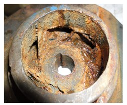
Two impellers ( 220 mm) were used. One impeller was assumed to be free from defect. The other impeller was prepared from an out-of-service pump. This impeller was rusted and the corrosion existed at the surface and the eye of the impeller as shown in Fig. 5.
Fig. 3Experimental setup
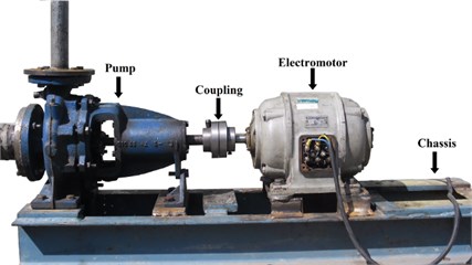
Fig. 4Location of the sensor
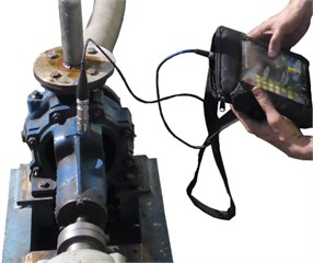
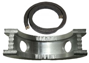
Fig. 5a) Faulty seal, b) faulty impeller
a)
b)
3.1.2. Fault in sealing system
Packing’s are one of the oldest sealing devices, named for the way they perform the sealing function. Packing is a rope-like material that is inserted into the cylindrical opening in the rear of the pump casing where the shaft passes through it. This soft material, usually with lubricant in it, consists of a number of rings that wrap around the shaft and compress the inner sides of the stuffing box. This effectively limits leakage out of the pump. The bronze component that separates the two sets of packing is called a lantern ring. The bronze lantern ring serves a number of functions inside the pump packing. The lantern ring is grooved with an oil groove and drilled with holes to allow lubrication to reach the packing material. The lantern ring is also used to distribute cooling water to all packing rings as well as keep the stuffing box clean of containments. Faulty packing was used to reduce the pressure of the pumped liquid and maximize leakage. Sometimes gland packing slightly swells on contact with water. This must be considered and an appropriate clearance should be provided. Otherwise, it would seize the shaft leading to overheating and burning of the packing. In some cases, the shafts have been even broken due to excessively tightened packing. Also, wear in the internal surface of the lantern ring makes friction and heat between the pump shaft and lantern ring, and destroys them. Heat and friction destroys pump shaft and lantern ring. Thus, in this study, we used a burned gland packing and a worn lantern ring, as shown in Fig. 5.
3.1.3. Cavitation
When a pump is under low pressure or high vacuum conditions, suction cavitation occurs. Thus, to simulate the cavitation, the valve at the inlet of the pump is used to make the pressure drop between the suction and the eye of the impeller. The valve control system is used to adjust the flow at the inlet and outlet of the pump. The control of priming and leakage of the pump was done. After closing the delivery valve, the pump started. Then the delivery valve was opened fully and the valve at the suction side was gradually closed. For more information on how to make cavitation, refer to [19].
3.2. Signal processing
As shown in Fig. 6, the collected signals of the first stage are in time domain. Before analyzing the signals, the samples were imported into MATLAB for preprocessing purposes, on each of which then the wavelet transform was applied using the Daubechies mother wavelet at three levels.
Fig. 6Vibration signals during different pump conditions; a) good condition; b) defect in seal; c) defect in impeller; d) cavitation
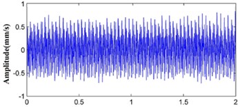
a)
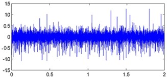
b)
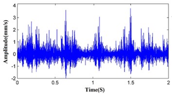
c)
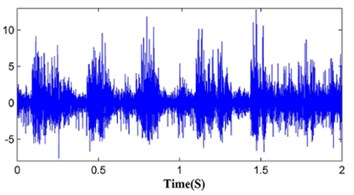
d)
3.3. Feature extraction and feature selection
In order to detect the symptoms for each of the faults in the centrifugal pump, the wavelet transform method was used for signal processing.
Vibration signals were processed by the WT at three levels of decomposition. Each signal was decomposed into one approximation signal and three detail signals. These signals are required to be transformed into usable forms; however, due to the large number of data for each fault, their processing procedure using conventional computers is a difficult and time-consuming task. To overcome the problem, 11 features from each coefficient of the wavelet transform were extracted. Mathematical equations of features are shown in Table 1. These features were extracted from Approximation3 (Ap3), Detail1 (De1), Detail2 (De2) and Detail3 (De3). Since each signal is subdivided into four auxiliary signals, 44 statistical features were extracted from each vibrational signal. However, since not all these features contain beneficial information, superior features should be selected as the input to the classifier. For this purpose, we used the correlation-based feature selection method as one of the most important feature selection techniques available in Weka software.
One hundred samples were collected for each of the pump conditions, 70 percent of which were used for training the SVM, and the remaining 30 percent for testing. The training and testing data were randomly selected, such that the SVM test was conducted using those data never exposed to the classifier.
Table 1Features and their equations used for feed classifier [11]
is a signal series for 1, 2, …, . is the number of data points |
4. Classification results using the SVM
The performance of the SVM depends on different factors including type of kernel function, penalty parameter, kernel parameter, and degree of a polynomial. In this study, one-vs-one classification was used to classify different conditions of the pump. In order to find the most appropriate model for classification of the faults in the centrifugal pump using the SVM, different parameters including penalty parameter (), degree of a polynomial () (increasing from 1 until the accuracy of the classifier decreases) and RBF kernel () were considered. Table 2 shows the classification results of the SVM for different values of the parameters. By changing the penalty parameter, the type of the kernel function and its degree, different classification percentages were obtained. The results revealed that the accuracy of the classifier increased as the penalty coefficient () decreased, such that the best results were obtained by changing 10 to 1, through which the accuracy of the SVM classifier increased by 10 percent. Moreover, the accuracy of the classifier increased as the degree of the polynomial increased, such that the maximum accuracy was obtained for a degree of 6. It should be noted that this is not always true, and better performances may be achieved for lower degrees. The most accurate results of fault classification using the SVM were obtained as 66.67 percent for a 6-degree kernel at a penalty coefficient of 1.
Fault classification using the SVM with the RBF kernel is given in Table 3 for different values of the penalty coefficient and kernel width. The results indicate that by decreasing the kernel width from 1 to 0.1, the accuracy of the SVM in detecting faults significantly increases, such that the best accuracy was obtained for a kernel width of 0.1. Similar to the previous results, the accuracy of the classifier increased with decreases in penalty coefficient. The best accuracy for fault classification using the SVM with the RBF kernel was obtained as 96.67 percent for a penalty coefficient of 1 and a kernel width of 0.1.
Table 2The accuracy of fault classification for a pump using a SVM with polynomial kernel
The penalty coefficient The kernel degree of the polynomial () | Classification accuracy (%) | ||
10 | 5 | 1 | |
1 | 50.00 | 50.00 | 53.33 |
2 | 50.00 | 53.33 | 56.67 |
3 | 53.33 | 56.67 | 56.67 |
4 | 53.33 | 60.00 | 60.00 |
5 | 56.67 | 63.33 | 63.33 |
6 | 56.67 | 53.33 | 66.67 |
7 | 50.00 | 53.33 | 56.67 |
8 | 50.00 | 53.33 | 56.67 |
Table 3The accuracy of fault classification for a pump using a SVM RBF kernel
The penalty coefficient RBF kernel Sigma parameter () | Classification accuracy (%) | ||
10 | 5 | 1 | |
0.1 | 93.33 | 93.33 | 96.67 |
0.2 | 93.33 | 93.33 | 93.33 |
0.3 | 90.00 | 93.33 | 93.33 |
0.4 | 90.00 | 93.33 | 93.33 |
0.5 | 86.67 | 86.67 | 90.00 |
0.6 | 83.33 | 86.67 | 90.00 |
0.7 | 83.33 | 86.67 | 86.67 |
0.8 | 77.67 | 83.33 | 86.67 |
0.9 | 77.67 | 77.67 | 86.67 |
1 | 75.13 | 76.33 | 77.67 |
Table 4Comparisons between the current work and some published work
References | Fault types | Classifier type | Classified states | Maximum classification efficiency (%) | Denoising technique | Feature selection method |
Yunlong and Peng [22] | IA, U, L | SVM | 4 | 92.60 | EMD | LS |
Sakthivel et al. [23] | BF, IF, SF, IBF, Ca | C4.5 decision tree algorithm | 6 | 100 | – | – |
Farokhzad et al. [11] | IF, SF, Ca | ANN | 4 | 100 | FFT | – |
Zouari et al. [33] | IA, Ca, PF, AI | ANN, FNN | 5 | 99.77 | – | PCA |
Muralidharan and Sugumaran [19] | BF, Ca, IF, IBF | J48 algorithm | 5 | 99.76 | WT | – |
Ebrahimi (Present work) | SF, IF, Ca | SVM | 4 | 96.67 | WT | CFS |
In order to illustrate the potential application of the proposed methodology in centrifugal pump fault diagnosis, a comparative study between the present work and published literature is presented in Table 4 [11, 19, 22, 23, 33]. The comparing items include the machine elements used, fault type, classifier type, classified states, maximum classification efficiencies, denoising technique and feature selection method. Therefore, the comparison results demonstrate that the proposed approach is effective and reliable in detecting centrifugal pump faults.
Also, the results of this study were in agreement with those of Konar [27], Yin and Hu [34] and, Bordoloi and Tiwari [35]. Comparison of the polynomial kernel method and the RBF kernel indicates that the RBF kernel has more accuracy for faults classification.
5. Conclusions
The aim of the present study was to use the wavelet transform and SVM to detect faults in centrifugal pumps. Five classical states viz., good condition, defect in seal, defect in impeller and cavitation, were simulated on the centrifugal pump. The vibration signals were decomposed by the Daubechies wavelets, and statistical features were extracted from the detail coefficients and approximation coefficients of the wavelet. Superior features should be selected as the input to the classifier. For this purpose, we used the correlation-based feature selection method as one of the most important feature selection techniques. Various parameters were used to increase the accuracy of the classifier, the effect of each of which is given in the following:
1) The accuracy of the classifier increased as the degree of kernel increased. However, this is not always true and lower degrees may result in better performances.
2) The accuracy of the classifier increased as the penalty coefficient () decreased, such that the best results were obtained by changing 10 to 1, through which the accuracy of the SVM classifier increased by 10 percent.
3) Reducing the width of the RBF kernel results in further accuracy of the classifier.
The best accuracy for fault classification using the SVM and RBF kernel was obtained as 96.67 percent for a penalty coefficient of 1 and a kernel width of 0.1. The results demonstrate that the proposed method can achieve good performance for fault detection of the centrifugal pump.
References
-
Yang M., Makis V. ARX model-based gearbox fault detection and localization under varying load conditions. Sound and Vibration, Vol. 329, Issue 24, 2010, p. 5209-5221.
-
Miao Q., Makis V. Condition monitoring and classification of rotating machinery using wavelets and hidden Markov models. Mechanical Systems and Signal Processing, Vol. 21, Issue 2, 2007, p. 840-855.
-
Niu G., Han T., Yang B. S., Tan A. C. C. Multi-agent decision fusion for motor fault diagnosis. Mechanical Systems and Signal Processing, Vol. 21, Issue 3, 2007, p. 1285-1299.
-
Wang X., Makis V., Yang M. A wavelet approach to fault diagnosis of a gearbox under varying load conditions. Sound and Vibration, Vol. 329, Issue 9, 2010, p. 1570-1580.
-
Sun H. C., Huang U. C. Support vector machine for vibration fault classification of steam turbine-generator sets. Procedia Engineering, Vol. 24, 2011, p. 38-42.
-
Bagheri B., Ahmadi H., Labbafi R. Implementing discrete wavelet transform and artificial neural networks for acoustic condition monitoring of gearbox. Elixir Mechanical Engineering, Vol. 35, 2011, p. 2909-2911.
-
Van Hecke B., Yoon J., He D. Low speed bearing fault diagnosis using acoustic emission sensors. Applied Acoustics, Vol. 105, 2016, p. 35-44.
-
Wu W., Lin T. R., Tan A. C. C. Normalization and source separation of acoustic emission signals for condition monitoring and fault detection of multi-cylinder diesel engines. Mechanical Systems and Signal Processing, Vols. 64-65, 2015, p. 479-497.
-
Yuan S., Chu F. Fault diagnosis based on support vector machines with parameter optimisation by artificial immunisation algorithm. Mechanical Systems and Signal Processing, Vol. 21, Issue 3, 2007, p. 1318-1330.
-
Wang J. D., Gao Y. Q., Zhao H. Y., Cong R. Sectional normalization and recognization on the PV Diagram of reciprocating compressor. Journal of Measurements in Engineering, Vol. 3, Issue 2, 2015, pp. 35 41.
-
Farokhzad S., Ahmadi H., Jaefari A., Asadi Asad Abad M. R., Ranjbar Kohan M. Artificial neural network based classification of faults in centrifugal water pump. Journal of Vibroengineering, Vol. 14, Issue 4, 2012, p. 1734-1744.
-
Yayli M. O. Free vibration behavior of a gradient elastic beam with varying cross section. Shock and Vibration, Vol. 2014, 2014, p. 801696.
-
Yayli M. O. On the axial vibration of carbon nanotubes with different boundary conditions. Micro and Nano Letters, Vol. 9, Issue 11, 2014, p. 807-811.
-
Hosseini A. H., Rahmani O., Nikmehr M., Golpayegani I. F. Axial vibration of cracked nanorods embedded in elastic foundation based on a nonlocal elasticity Model. Sensor Letters, Vol. 14, Issue 10, 2016, p. 1019-1025.
-
Yayli M. O. An analytical solution for free vibrations of a cantilever nanobeam with a spring mass system. International Journal of Engineering and Applied Sciences, Vol. 7, Issue 4, 2015, p. 10-18.
-
Li Y., Xu M., Wang R., Huang W. A fault diagnosis scheme for rolling bearing based on local mean decomposition and improved multiscale fuzzy entropy. Journal of Sound and Vibration, Vol. 360, 2016, p. 277-299.
-
Li Y., Xu M., Wei Y. An improvement EMD method based on the optimized rational Hermite interpolation approach and its application to gear fault Diagnosis. Measurement, Vol. 63, 2015, p. 330-345.
-
Li Y., Xu M., Wei Y., Huang W. A new rolling bearing fault diagnosis method based on multiscale permutation entropy and improved support vector machine based binary tree. Measurement, Vol. 77, 2016, p. 80-94.
-
Muralidharan V., Sugumaran V. Feature extraction using wavelets and classification through decision tree algorithm for fault diagnosis of mono-block centrifugal pump. Measurement, Vol. 46, Issue 1, 2013, p. 353-359.
-
Kiran V., Hemantha K., Gangadharan K. V. Gear fault detection using vibration analysis and continuous wavelet transform. Procedia Materials Science, Vol. 5, 2014, p. 1846-1852.
-
Li Y., Yang Y., Li G., Xu M., Huang W. A fault diagnosis scheme for planetary gearboxes using modified multi-scale symbolic dynamic entropy and mRMR feature selection. Mechanical Systems and Signal Processing, Vol. 91, 2017, p. 295-312.
-
Yunlong Z., Peng Z. Vibration fault diagnosis method of centrifugal pump based on EMD complexity feature and least square support vector machine. Energy Procedia, Vol. 17, 2012, p. 939-495.
-
Sakthivel N. R., Sugumaran V., Babudevasenapati S. Vibration based fault diagnosis of monoblock centrifugal pump using decision tree. Expert Systems with Applications, Vol. 37, Issue 6, 2010, p. 4040-4049.
-
Cui H., Zhang L., Kang R., Lan X. Research on fault diagnosis for reciprocating compressor valve using information entropy and SVM method. Journal of Loss Prevention in the Process Industries, Vol. 22, 2009, p. 864-867.
-
Zhao G., Jiang D., Diao J. Application of wavelet time-frequency analysis on fault diagnosis for steam turbine. 5th International Conference Acoustical and Vibratory Surveillance Methods and Diagnostic Techniques, Senlis, France, 2004.
-
Jedlinski L., Jonak J. Early fault detection in gearboxes based on support vector machines and multilayer perceptron with a continuous wavelet transform. Applied Soft Computing, Vol. 30, 2015, p. 636-641.
-
Konar P., Chattopadhyay P. Bearing fault detection of induction motor using wavelet and support vector machines (SVMs). Applied Soft Computing, Vol. 11, Issue 6, 2011, p. 4203-4211.
-
Choudhury M., Ganguly A. Transmission line fault classification using discrete wavelet transform. International Conference on Energy, Power and Environment: Towards Sustainable Growth (ICEPE), 2015.
-
Bendjama H., Bouhouche S., Boucherit M. S. Application of wavelet transform for fault diagnosis in rotating machinery. International Journal of Machine Learning and Computing, Vol. 2, Issue 1, 2012, p. 82-87.
-
Cristianini N., Taylor J. S. An Introduction to Support Vector Machines and Other Kernel-Based Learning Methods. Cambridge University Press, 2000.
-
Bioinformatics Toolbox, Getting Started, Support Vector Machine (SVM). Matlab Help, 2011.
-
Shen L., Chen H., Yu Z., Kang W., Zhang B., Li H., Yang B., Liu D. Evolving support vector machines using fruit fly optimization for medical data classification. Knowledge-Based Systems, Vol. 96, Issue 15, 2016, p. 61-75.
-
Zouari R., Sieg-Zieba S., Sidahmed M. Fault detection system for centrifugal pumps using neural networks and neuro-fuzzy techniques. Surveillance 5 CETIM, Senlis, 2004.
-
Yin Z., Hou J. Recent advances on SVM based fault diagnosis and process monitoring in complicated industrial processes. Neurocomputing, Vol. 174, 2016, p. 643-650.
-
Bordoloi D. J., Tiwari R. Optimum multi-fault classification of gears with integration of evolutionary and SVM algorithms. Mechanism and Machine Theory, Vol. 73, 2014, p. 49-60.
About this article

This research is supported by the Islamic Azad University, Kermanshah Branch, Iran. This assistance is gratefully appreciated.
