Abstract
The purpose of this work is to develop a mathematical model of the dynamics of turning a thin-walled cylindrical shell. This model uses a finite number of degrees of freedom and takes into account the variability of dynamic compliance. It is then possible to obtain estimates of the boundaries of stability of the continuous cutting process. The model is based on the theory of shells with application of Galerkin’s method in conjunction with the expansion of the displacement field in beam and trigonometric functions. On the basis of the developed model, an algorithm designed for constructing boundaries of stability of turning of the thin-walled cylindrical parts is presented and compared to experimental results. A strategy to define matter removal sequences is proposed.
1. Introduction
Investigating the stability of the cutting process has been the subject of studies for many years now. The first works appeared at the beginning of the 50s and explained the basic mechanism of occurrence of self-oscillations in the machining process “over the trace on the previously cut surface”. Currently, this effect is considered the main cause of chatter vibrations. This regenerative mechanism of excitation of oscillations is widely used in the method of analysis of the stability of the stationary cutting process. This method is based on the analysis of the characteristic equation with the further construction of the stability diagram [1, 2]. Most of the works devoted to the study of the stability of the process of turning use as an object a cylindrical full workpiece [3, 4] or beams [5, 6]. However, in [7], the author conducted an experiment of turning thin-walled cylindrical part and showed the presence of areas that were vibrating during the process. More recently a stability study of turning aluminum tubes, finite element modeled, for a variety of processing conditions was carried out [8, 9]. A time domain simulation of the turning process is presented in [10] where the influence of damping on emergence of unstable cutting process was shown. All these works show the influence of damping on the occurrence of vibrations during cutting. Another feature of the turning of thin-walled cylindrical parts is a strong change in the dynamic stiffness and in the natural frequencies of the workpiece during the pass.
In this paper, the turning of a thin-walled cylindrical shell using an analytical approach to model the dynamics is studied. This analytical approach is based on the Kirhgoff-Love shell theory. The assumption of the middle surface inextensibility is used [11]. The system of differential equations of dynamics of the shell, expressed in terms of the axial, circumferential and radial components of displacement, was conducted by using variational principles. The research of solutions of this system is performed by Fourier expansion of the components of displacement along the circumferential direction and beam functions in axial direction [12-14] and uses the Galerkin’s method [15-17]. The obtained analytical model allows estimating the boundaries of stability zones for the continuous cutting process. It takes into account the continuous changing of dynamics due to matter removal and motion of the tool over a flexible part. An experimental validation is presented and a strategy to optimize the turning process is proposed.
In Section 2, we present the analytical model that contains a finite number of degrees of freedom. In Section 3 we present the way we use to estimate the stability of the process and in Section 4 we describe the design of the experiment uses for validation. The experiment was chosen in order to have an increase in compliance of workpiece while the tool progresses until chatter occurs. A presentation of the obtained results and a discussion are given in Section 5. Finally, a way to optimize to sequence of tool passes is proposed in Section 6. The conclusions take place in Section 7.
2. Analytical simulation of the turning process
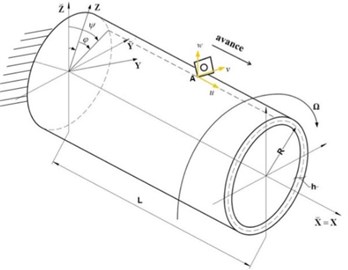
A cylindrical thin-walled shell (Fig. 1) is considered. The shell is in rotation around its axis at a constant angular velocity . The shell is loaded with a moving force, the cutting force, which has, with respect to the shell, an angular velocity –. The left edge of the shell is fixed, the right one is free. The geometric parameters of the shell are , which account for length, radius and thickness, respectively.
The following coordinates systems (see Fig. 1) are used: mobile system of coordinates, linked to the rotating part; fixed system of coordinates, connected to the frame of the machine tool.
Fig. 1Schema of the model
2.1. Basic system of equations of the thin-walled shell
The system of differential equations of dynamics of the shell, expressed in terms of the components , , , on axial, circumferential and radial displacement, can be represented as the follows [18]:
The expression of the differential operators are:
where denotes the partial derivative with respect to , , , represent the components of the surface forces acting on the shell in the axial, circumferential and radial directions, respectively.
The rotation-induced load terms are expressed as follows:
As shown in [19], these components have a small impact on the dynamics of the shell, and can be neglected in further calculations.
The components of the surface forces, applied to the shell, modelled by an interaction with the tool, are expressed as follows:
where , are the coordinates of the position of the tool, in the mobile frame, in axial and circumferential direction, respectively (both are time dependent); refers to the components of the external point cutting force, is the Dirac function.
2.2. Model of the cutting force
In this work, a linear cutting law (cutting force model), linearized around the nominal cutting parameters, is used. Therefore, the force, which models the effect of the tool on the shell for each direction, is expressed as follows:
where is the coefficient of cutting stiffness, is the cutting force in nominal conditions, represents dynamic perturbation of the cutting depth, due to vibrations, is the period of rotation and , , are the direction cosines of the force vector.
To study the stability of the cutting process, the system is considered in a perturbed state and therefore the part of the cutting forces associated with the perturbation, which is used, can be written as follows:
2.3. Discretization of the system of equations
In order to find the solution of the Eq. (1), a Fourier expansion of the components of displacement along the axial and circumferential coordinate is carried out, with the further use of the Galerkin’s method.
The displacement field is written as follows:
where , , are the unknown axial basic functions, is the number of harmonics in the circumferential direction, is the number of harmonics in the axial direction, , are unknown amplitude functions of time.
The axial basic functions are beam functions written as follows [14, 15, 20]:
The parameters , , , , are determined according to a set of boundary conditions.
The relationship between functions is determined by the state of non-extensible middle surface, namely , [11].
According to boundary conditions, at hand clamped-free, the function will have the following form [14, 15, 20]:
Note that the , do not depend on the number of circumferential harmonics .
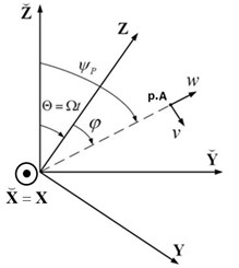
The final system of equations of motion of the shell is presented in the fixed coordinate system , , , because of simplicity of representation of the point of interaction (point A, Fig. 2) between the tool and the shell for further analysis of stability.
The components of displacement of the shell in the moving frame are , , and , , are the components of this displacement in the fixed frame. The angle gives the position of the tool in the fixed frame. This angle is not time dependent.
Fig. 2Relation between the different coordinate systems
2.4. Writing systems in matrix form
The final system of differential equations of dynamics of the shell is written in matrix form for the unknown amplitude dimensionless variables , depending on the time and for one particular circumferential harmonic :
The vector of solution in Eq. (10) consists of a set of vectors for each axial harmonic and one particular circumferential harmonic , and these vectors consist of a set of symmetric and antisymmetric amplitude components:
where , are unknown amplitude functions of time.
The vector of load (dimension ) is written:
The matrices , , are derived via Galerkin method. Their structures and their components can be found in the appendix. All these matrices are dependent on the tool position along the axial coordinate . Changes in the thickness of the shell is taken into account with the help of the integrals Eq. (29). Also, dynamic compliance variation of the cutting process is taken into account by changing the position of the tool Eq. (32).
The matrix is determined with help of the Rayleigh damping model:
The constant of Rayleigh , have been determined from experimental results given in Table 2 In the present case we have , for , and their corresponding frequencies Hz, Hz.
The system of Eq. (10) describes the turning process of a thin-walled cylindrical shell whose interaction with the tool is defined by a cutting force concentrated on a mobile point.
3. Stability evaluation of cutting process
The stability of the turning process is investigated, using the previous model and the procedure described in the book of Cheng [2].
The solution of Eq. (10) will be sought in the form:
After substituting Eq. (14) into Eq. (10), the following equation is obtained:
where:
At the boundaries of the stability areas, the is purely imaginary. So, the critical parameters of the cut are found via characteristic Eq. (15):
By substituting , the characteristic equation is divided in real and imaginary parts. The parameter represents the oscillation frequency at the limit of the zone of stability, when the characteristic factor becomes purely imaginary. Subsequently, the oscillation frequency will be called chatter frequency.
It is possible to combine the eigenvalues of Eq. (17) into a vector . Each component of this vector leads, according to Eq. (16), to the resolution of:
where is the component of the eigenvalues vector, which is determined from the solution of the eigenvalue problem, i.e The coefficients and represent the real and imaginary components of .
This leads to:
The Eq. (19) is divided in the real part and imaginary part:
From the resulting system of Eq. (20), the stiffness of cutting is expressed [2]:
and also [22]:
where is the angle phase.
The number of oscillation per revolution [14] is given by:
where , are the integer and the fractional number of incisions on the surface, respectively.
Taking into account Eqs. (22) and (23) leads to:
The solution of Eq. (20) is a pair of parameters for each set of frequency value and position of the tool , where the parameters , are arbitrary constants.
This approach gives place to the following algorithm:
• On the first step of the algorithm, the frequency parameter is fixed (the smallest eigenvalue of the eigenvalue problem of conservative system ).
• In a second step, the eigenvalue problem is solved, namely , , from which the vector of eigenvalues is determined.
• Then, for each eigenvalue , using the Eqs. (21), (22) and (24), the following parameters , and are calculated. The final step enables to calculate the period of rotation .
• The cycle is repeated for the next value of the frequency parameter (where is an arbitrary constant).
The obtained data set enables the drawing of a multi-Dof lobe stability diagram.
4. Experimental setup and measurements
As an illustration of the above designed approach, an experiment has been carried out, namely. The turning of the outer cylindrical surface of a tubular part, as can be seen on the drawing (Fig. 3), was conducted. The experimental set up consists of a part, fixed by a three-jaw chuck to the machine tool spindle, and a set of sensors. This experiment has been partly addressed in [21, 22].
In the framework of the experiment, several types of sensors were used. The experimental set up is shown in Fig. 4. For the vibration measurement of the workpiece two types of sensor are used: i) displacement eddy current sensors (3a, 3b, Fig. 4) and ii) accelerometers (2a, 2b, 2c, 2d, Fig. 4). For the measurement of the frequency of rotation of the workpiece an optical sensor was used (1a, Fig. 4).
On Fig. 4, one can also see the eddy current sensor ’3a’ but, due to presence of chips inside the tube, it was not exploitable. The accelerometer ’2c’ was positioned on ’3a’ sensor support to measure the vibrations of this support.
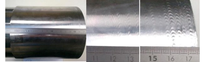
The pass of the tool is repeated several times until occurrence of vibrations of large amplitudes generating significant damage on the machined surface. The generated defects on the machined surface during the last tool pass are shown on Fig. 5. This occurred for a thickness of the tube going from 5.4 mm to 4.4 mm.
Fig. 3Geometry of the machined tube
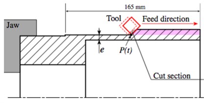
Fig. 4Experimental setup
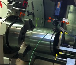
Fig. 5Surface of the tube after the last tool pass
An impact test was carried out before and after the machining. The main aim of this test was the definition of modal characteristics of the workpiece before and after the turning process. The respective transfer functions are presented on Fig. 6. The experimental data given in Table 1 and Table 2 are coming from these transfer functions.
Fig. 6Transfer function before and after the last tool path
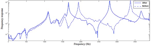
Table 1Experimental eigenfrequencies before the passage of the tool
Freq. experiment (Hz) | 1108.4 | 1937.2 | 3384.5 |
Modal Damping | 0.0105 | 0.0076 | 0.00051 |
Modal form | 2 lobes | 3 lobes | Flexion 2 |
Table 2Experimental eigenfrequencies after the passage of the tool
Freq. experiment (Hz) | 1100.2 | 1661.1 | 2798 |
Modal Damping | 0.0077 | 0.00070 | 0.00078 |
Modal form | 2 lobes | 3 lobes | 4 lobes |
The signal of the eddy current sensor ’3b’, fixed on the machine frame, is presented on Fig. 7. This sensor is placed in front of the right extremity of the workpiece where the largest displacements are present.
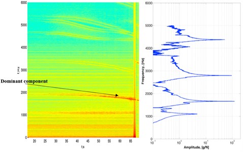
On the right side () of the graphic (Fig. 7) the observed oscillations correspond to those visible on the workpiece surface on Fig. 5. On the spectrogram computed from this displacement signal (Fig. 8) one can see the evolution of the resonances of the tube close to the evolution of its eigenfrequencies. On the right of the Fig. 8 the result of the hammer test after the last tool pass is given (solid line from Fig. 6).
And, as shown by the analysis of the spectrogram and FRF (Fig. 8), the dominant vibration component is close to a natural frequency of the workpiece.
Fig. 7Signal recorded using the sensor 3b
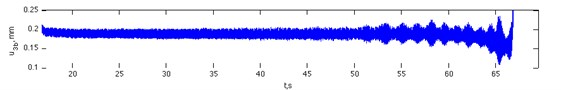
Fig. 8Spectrogram issued from the measurement of the eddy current sensor ’3b’ with the result of hammer test after the final pass
5. Results and discussion
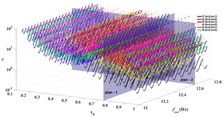
As previously said, the solution of Eq. (20) is the pair of parameters for each frequency value and depends on the tool position . We build the stability curves for different positions of the tool , with the following notations: cutting stiffness coefficient and rotation frequency , with: – cutting stiffness of the system, [N/m]; – nominal cutting stiffness, obtained from experiment (here, 569 N/m), for the tool-workpiece set studied, [N/m];
The Fig. 9 shows the three-dimensional stability diagram of the continuous cutting process in the three-parameter space . This graph shows that conditions of stability change, depending of the tool position. The number of different degrees of freedom in the system considered is the number of sets of lobes representing the limits of stability, highlighted by different colors.
Fig. 9Stability diagram in the parameter space xP,κ,frot
The Fig. 10(а) represents a clipping plan of the stability diagram in the two-parameters plane, for the position of the tool . It corresponds to the loss of stability of the quasi-static cutting process. For the considered state of the system, and the specified range of technological parameters, three sets of lobes are obtained, each of the sets having a different color. In practice, the border of the lower zone of stability is our only concern because, from the moment the parameters of the system reach the lower stability boundary, the continuous cutting process becomes unstable. The red vertical line represents the rotation frequency of the workpiece, corresponding to the experiment Hz. On the same line, corresponding to the rotational frequency of interest, there are several different sets of lobes representing a limit of the stability zone. The red vertical line intersects the first set of lobes in point А. To evaluate the stability of the quasi-static cutting process, the relative position of the point А (the intersection point of the rotational frequency of interest with the lowest set of lobes representing the border of the stability area) has to be estimated by comparing it to the limit value of the cutting stiffness coefficient (horizontal blue line). If the point A is above the blue line, then the quasi-static cutting process is stable. If it is below the blue line, the process is unstable. Fig. 10(a) shows that the quasi-static cutting process is located on the border of the zone of stability. One of the characteristics of the boundary of the stability zone of the cutting process consists in the oscillation frequency, called chatter frequency. It is at this frequency that the self-excited oscillations of the system begin, if the process parameters are within the instability area of the system. The chatter frequency may vary depending on the encountered stability zone and on the positions with respect to this zone. On the Fig. 10(b) is shown the variation of the critical stiffness parameter of the system depending on the chatter frequency .
To determine the chatter frequency, which corresponds to the oscillation frequency on the border of the zone of stability for the rotational frequency considered, the value of parameter must be known at the intersection with the boundary of the zone of stability at the relevant rotational frequency (the point А, Fig. 10(а)). For the lowest limit of the stability area, which corresponds to the black lines in Fig. 10(a), the value of the parameter is (Fig. 10(а)). Then, reporting this value on the Fig. 10(b), the value of the chatter frequency is obtained: Hz. This means that at the limit of the zone of instability self-oscillations begin to develop at the frequency Hz. It is important to note that each set of boundaries of the stability area has its own chatter function, as shown on Fig. 11(a) and Fig. 11(b).
The stability boundaries for the position of the tool in the plane of parameters are presented on Fig. 11(a). There are 6 families of these boundaries in total (each assigned with a different color). On Fig. 11(b), for this position of the tool and this field of parameter , the evolution of the stiffness parameter of the system , depending on the chatter frequency, is plotted. The 6 sets of different limits of stability zone are clearly seen, in different colors (Fig. 11(а)), and each set has its own function of chatter frequency (Fig. 11(b)). Thus, each set of lobes has its own variation of the stiffness parameter of cutting and of the chatter frequency during the process. The lowest boundary of stability at given for the position of the tool is the set of lobes shown in blue (Fig. 11(а)).
Fig. 10Clipping plane of the stability diagram in the κ,frot and κ,fchat planes, for the tool position xp=0.739L
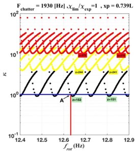
a) Variation of the as a function of the workpiece rotational frequency
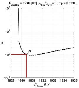
b) Variation of the with respect to the chatter frequency
Fig. 11Clipping plane of the stability diagram in the plans κ,frot and κ,fchat for the tool position xP=0.574L
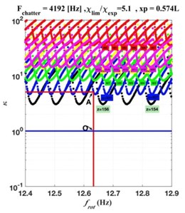
a) Variation of the as a function of the workpiece rotational frequency
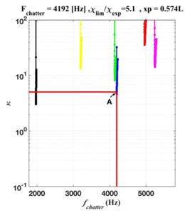
b) Variation of the with respect to the chatter frequency
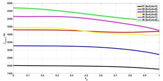
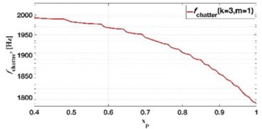
The frequency of oscillations on the stability boundary shows some variations, depending on the position of the tool (Fig. 12). The values shown in this diagram correspond to the frequency values, obtained by the intersection of the vertical line of the rotational frequency with the boundaries of stability regions for each of the positions of the tool. It was found that the frequencies at the boundaries of stability domains are very close to the natural frequencies of the shell.
Fig. 12Variation of the frequency of oscillations on the border of the zone of stability depending on the position of the tool
During the pass of the tool, a chip has been removed, thus leading to modifications in the dynamic characteristics of the system, including the natural frequencies of the shell. The results obtained by modeling the system during the 16th pass of the tool can be compared with the experimental data (Fig. 13).
During the experiment, it was observed that the system responded for some frequencies (Fig. 13(а)). In the range of 0-6000 Hz, there are 6 frequencies that lead to a response of the system.
The spectrogram during the final pass of the tool is presented on Fig. 13. The frequencies, which lead to a response of the system when the tool passes on the shell, are shown in red and numbered (Fig. 13(а)). The oscillation frequencies, shown in black and numbered on the borders of the stability areas of the continuous cutting are obtained by calculation (Fig. 13(b)). When crossing the border of the stability area of the limit stiffness parameter , one of the oscillation frequencies becomes the chatter frequency, from which begins the process of self-excited oscillations.
Fig. 13Comparison between the chatter frequency of the experiment and the frequencies calculated using the analytical model
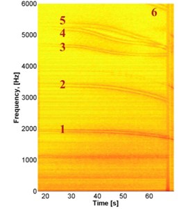
a)
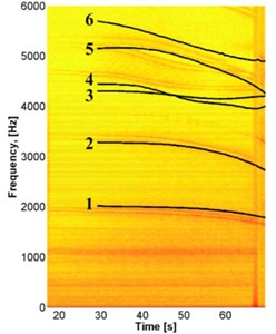
b)
The chatter frequency that dominates at the end of the pass in the experiment is 1670 Hz. The frequencies numbered 1, 2, 3 and 5 are close to the experimental result, with an error below 5 %, while the frequencies 4 and 6 are assigned with an error of 15 to 17 %. This difference shows that for , which is the number of axial harmonics that we use for the approximation Eq. (7) introduced in the Galerkin method, is much better for modes whose axial form is close to the first harmonic () than for the modes whose axial shape is close to the second harmonic (). It is possible to improve this result if we take . Nevertheless, the chatter frequency, which is 1670 Hz and corresponds to the loss of stability, is well described by this model.
The inferred chatter frequency variation alongside the instability zone number 153 change (Fig. 15), results in a discontinuous chatter frequency evaluation. This is in qualitative agreement on the observed stairs-like pattern in the signal spectrum, as shown on Fig 14.
Fig. 14Comparison of the chatter frequency
a) Computed for lowest critical stifness
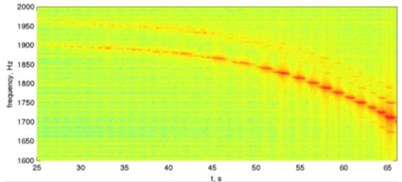
b) Spectrogram detailed for the frequency that dominates the response
Fig. 15Critical relative rigidity of the system variation during the pass
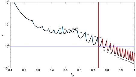
Fig. 15 shows a sectional view of the stability diagram in three dimensions (plans – 2, Fig. 9) in the parameter area . On this diagram, one can see how the limit stiffness of the system changes during the pass of the tool and therefore when the nominal cutting process becomes unstable.
Fig. 15 shows only the lower limit of the zone of stability (for the studied rotational frequency), because ultimately it is the only important one for the stability analysis of the cut. As can be seen, the first loss of stability of the cutting process takes place when the tool is at position . The stability diagram for this position of the tool in the parameters area is shown in Fig. 10.
6. Optimizing the operations of turning
Our approach allows estimating the boundary conditions of the cutting for each pass of the tool, which lead the turning process to the vibrations. So, using this information, an estimation of the maximum cutting depth for each pass can be made, for which the cutting will take place without chatter. For example, in the experiment presented above, the last pass should have a cutting depth limit below mm. Thus, in order to avoid vibrations during the turning process, the remaining passes and the depth of cut should be determined on the basis of this finding.
Table 3 presents a strategy of the turning without vibration to produce a part having a final thickness of mm.
The cutting depth specified is the maximum allowed for each of the passes, in order to determine the fastest way to get the piece with a specified wall thickness without vibration. These parameters are determined from the last pass to the first one. This means that the maximum cutting depth for each (current) pass depends on the conditions of the following passes.
Based on the approach described above, a diagram of the turning sequence can be worked out (Fig. 16).
Table 3Technological plan of the turning without vibration
Number of the pass | Thickness before the pass , (mm) | Thickness after the pass , (mm) | Cutting depth limit , (mm) |
N-5 | 7,7 | 6,9 | 0,81 |
N-4 | 6,9 | 6,2 | 0,68 |
N-3 | 6,2 | 5,6 | 0,57 |
N-2 | 5,6 | 5,1 | 0,47 |
N-1 | 5,1 | 4,7 | 0,38 |
N | 4,7 | 4,4 | 0,3 |
Fig. 16Limit thickness sequence diagram of the turning
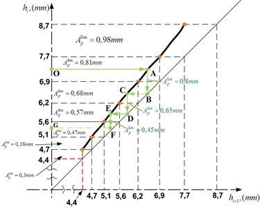
This diagram is drawn along the axes and , which represent the current wall thickness and the future one, respectively. This plot can not only be used for the point values from Table 3, but can also be practical for intermediate values via interpolation.
For example, for a piece with an initial thickness of mm, a piece with a final wall thickness of mm is obtained. The horizontal segment OA of the diagram shows the initial thickness of the piece, this segment goes through the black line at point A, and from the intersection point, draws a vertical segment , thus leading to the maximum cutting depth, which is mm for the first pass. The segment mm illustrates the cutting depth limit for the second pass. For the third and final pass, the cutting depth is mm, from which a piece with a mm wall thickness is obtained, illustrated by the segment .
7. Conclusions
A mathematical model of the turning was proposed and developed, with a finite number of degrees of freedom for a reliable estimate of the limits of stability of the continuous cutting. Based on the proposed model, an algorithm was developed to define the limits of the stability regions of the turning process of a thin-walled cylindrical part. It is shown that the boundaries of the stability zones of the cutting process occur at oscillation frequencies close to the natural frequencies of the part. The importance of the use of models with several degrees of freedom is enhanced by the fact that, upon progression of the tool, the dynamic characteristics of the part may vary, in particular, the vibration modes and its Eigen frequencies, which can lead to significant changes within the areas of instability. Since the frequency at which the stability of the cutting process will be lost is not known a priori, as well as the form of vibration corresponding to this frequency, several modes must be taken into account. Thus, with the help of the limit thickness sequence diagram, some recommendations on the choice of technological parameters of the cutting were made, for the turning, to avoid the vibrations observed during the cutting process and to get the final result as rapidly as possible.
References
-
Altintas Y. Manufacturing Automation: Metal Cutting Mechanics. Machine Tool Vibrations, and CNC Design. Cambridge University Press, 2012.
-
Cheng K. Machining Dynamics: Fundamentals, Applications and Practices. Springer, 2008.
-
Urbikain G., López de Lacalle L. N., Campa F. J., Fernández A., Elías A. Stability prediction in straight turning of a flexible workpiece by collocation method. International Journal of Machine Tools and Manufacture, Vol. 54, Issue 55, 2012, p. 73-81.
-
Zoltan Dombovari, Barton David A. W., Wilson R. Eddie, GaborStepan On the global dynamics of chatter in the orthogonal cutting model. International Journal of Non-Linear Mechanics, Vol. 46, Issue 1, 2011, p. 330-338.
-
Chen C. K., Tsao Y. M. A stability analysis of turning a tailstock supported flexible work-piece, International Journal of Machine Tools and Manufacture, Vol. 46, 2006, p. 18-25.
-
Chen C. K., Tsao Y. M. A stability analysis of regenerative chatter in turning process without using tailstock. The International Journal of Advanced Manufacturing Technology, Vol. 29, 2006, p. 648-654.
-
Arnold Rn Chatter patterns formed on the surface of thin cylindrical tubes during machining. Journal of Mechanical Engineering Science, Vol. 3, 1961, p. 7-14.
-
Mehdi K., Rigal J., Play D. Dynamic behavior of a thin-walled cylindrical workpiece during the turning process, Part 2: Experimental approach and validation. Journal of Manufacturing Science and Engineering, Vol. 124, Issues 3-569, 2002, p. 580-11.
-
Mehdi K., Rigal J., Play D. Dynamic behavior of a thin-walled cylindrical workpiece during the turning process, Part 1: Cutting process simulation. Journal of Manufacturing Science and Engineering, Vol. 124, Issue 3, 2002, p. 569-580.
-
Lorong P., Larue A., Duarte A. P. Dynamic materials research. Advanced Materials Research, Vol. 223, 2011, p. 591-599.
-
Matveyev V. A., Lipatnikov V. I., Alekhin A. V. The Designing of Wave Horoscope. MGTU, 1997, (in Russian).
-
Lam K. Y., Loy C. T. Effects of boundary conditions on frequencies of a multilayered cylindrical shell. Journal of Sound and Vibration, Vol. 188, Issues 3-7, 1995, p. 363-384.
-
Zhang X. M., Liu G. R. Vibration Analysis of thin cylindrical shells using wave propagation approach. Journal of Sound and Vibration, Vol. 239, Issue 3, 2001, p. 397-403.
-
Blevins R. D. Formulas for Natural Frequency and Mode Shape. Van Nostrand Reinhold, New York, 1979.
-
Li Hua, Lam Shin-Yong Rotating shell dynamics. Studies in Applied Mechanics, Vol. 50, 2005, p. 284.
-
Lopatin A. V., Morozov E. V., Shatov A. V. An analytical expression for fundamental frequency of the composite lattice cylindrical shell with clamped edges. Composite Structures, Vol. 141, 2016, p. 232-239.
-
Jam J., Zadeh M., Taghavian H., Eftari B. Vibration analysis of grid-stiffened circular cylindrical shells with full free edges. Polish Maritime Research, Vol. 18, Issue 4, 2011, p. 23-27.
-
Biderman V. L. Mechanics of Thin-Walled Structures. Mashinostroyeniye, 1977, (in Russian).
-
Gerasimenko A. A., Gouskov A. M. Determination of the Natural Frequencies of the Rotating Cylindrical Shell. Mashinostroyeniye, 2012, (in Russian).
-
Kolkunov N. V. Basis of Calculation of the Elastic Shells. 2d. Edition, High School, 1972, (in Russian).
-
Gerasimenko A., Guskov M., Lorong P., Duchemin J., Gouskov A. Experimental investigation of chatter dynamics in thin-walled tubular parts turning. Procedia CIRP, 2016.
-
Gerasimenko A., Guskov M., Duchemin J., Lorong P., Gouskov A. Variable compliance-related aspects of chatter in turning thin-walled tubular parts. Procedia CIRP, Vol. 31, 2015, p. 58-63.
-
Altintas Y. Manufacturing Automation. Metal Cutting Mechanics, Machine Tool Vibrations, and CNC Design. Cambridge University Press, Cambridge, 2000.
-
Bolotin V. V. Vibrations in the Techniques. Mashinostroenie, 1978, p. 352, (in Russian).
Cited by
About this article

The research was funded by the financial support of Ministry of Education and Science, NIR No. 9.1073.2014K under the design part of the State-guaranteed order in scientific research area. The work was carried out with the financial support of the RFBR grant (Project No. 16-58-150001 NCNI_a).
A. Gouskov and P. Lorong: joint discussion to set research goals, choice of the analysis method for the calculation, joint discussion of the results of calculations and experiments, carried out the experiments. A. Gerasimenko, M. Guskov and A. Shokhin: preparation of the experiments, carried out the experiments, carried out the calculation, treatment of the results of experiments and calculation, joint discussion of the results of calculations and experiments.
