Sparse decomposition based on ADMM dictionary learning for fault feature extraction of rolling element bearing

Tong, Qingbin; Sun, Zhanlong; Nie, Zhengwei; Lin, Yuyi; Cao, Junci

doi:10.21595/jve.2016.17566

Journal of Vibroengineering

Browse Journal

Submit article

Published: 31 December 2016

Check for updates

Sparse decomposition based on ADMM dictionary learning for fault feature extraction of rolling element bearing

Qingbin Tong¹

Zhanlong Sun²

Zhengwei Nie³

Yuyi Lin⁴

Junci Cao⁵

^{1, 2, 3, 5}School of Electrical Engineering, Beijing Jiaotong University, Beijing 100044, China

^{4, 3}Department of Mechanical and Aerospace Engineering, University of Missouri, Columbia MO 65211, USA

Corresponding Author:

Qingbin Tong

Cite the article Download PDF

Downloads 1738

WoS Core Citations 6

CrossRef Citations 4

Abstract

Sparse decomposition is a novel method for the fault diagnosis of rolling element bearing, whether the construction of dictionary model is good or not will directly affect the results of sparse decomposition. In order to effectively extract the fault characteristics of rolling element bearing, a sparse decomposition method based on the over-complete dictionary learning of alternating direction method of multipliers (ADMM) is presented in this paper. In the process of dictionary learning, ADMM is used to update the atoms of the dictionary. Compared with the K-SVD dictionary learning and non-learning dictionary method, the learned ADMM dictionary has a better structure and faster speed in the sparse decomposition. The ADMM dictionary learning method combined with the orthogonal matching pursuit (OMP) is used to implement the sparse decomposition of the vibration signal. The envelope spectrum technique is used to analyze the results of the sparse decomposition for the fault feature extraction of the rolling element bearing. The experimental results show that the ADMM dictionary learning method can updates the dictionary atoms to better fit the original signal data than K-SVD dictionary learning, the high frequency noise in the vibration signal of the rolling bearing can be effectively suppressed, and the fault characteristic frequency can be highlighted, which is very favorable for the fault diagnosis of the rolling element bearing.

1. Introduction

Rolling element bearings are regarded as one of the most common components in rotating machinery of modern industry. The failure of rolling element bearings can result in the deterioration of machine operating conditions after a long-term running in the complex and severe conditions such as high speed, heavy load, strong impact or high temperature environment [1, 2]. Therefore, reliable bearing fault detection techniques are very significant to recognize a bearing defect at its earliest stage so as to prevent machinery performance degradation and malfunctions. Bearing fault detection can be undertaken using different information carriers such as vibration signals, lubricant information, and acoustic and temperature data [3]. Among them, vibration signals carry rich condition-related information due to the fact that a series of impact impulses will occur when a rolling element bearing hits a localized fault [4, 5]. Therefore, vibration-based analysis is mostly commonly applied in the condition monitoring and fault diagnosis of rolling element bearings [6-8]. Nevertheless, in practice the defect-induced impulses are often too weak to be distinguished in the complex data corrupted by a large amount of background noise. Therefore, it is critical to denoise the raw measured signals and extract intrinsic transient characteristics for the fault diagnosis of rolling element bearing at early stages.

To effectively extract the fault feature from the vibration signals, various techniques have been developed for the fault diagnosis of rolling element bearing, such as Wigner-Viller distribution (WVD) [9], the wavelet transform (WT) [10], the empirical mode decomposition (EMD) [11, 12], the local mean decomposition (LMD) [13, 14], etc. However, traditional methods based on orthogonal linear transforms are not suitable for the multiple components present in the natural complex vibration signals. Sparse representations of signals have received a great deal of attentions in recent years for the fault diagnosis of rolling element bearing [15-17]. Different from the traditional orthogonal basis transformation, the problem solved by the sparse representation is to search for the most compact representation of a signal in terms of linear combination of atoms in an over-complete dictionary [18]. Sparse representation can be served as the decomposition and reconstruction problems. Sparse decomposition mainly consists of two aspects: one type focus on the algorithm optimization and improvement for representing the signal by learned sparse components or sparse atoms, and the other type is on the atom function modeling for an over-complete dictionary construction. Therefore, successful application of a sparse decomposition depends on the dictionary used, and whether it matches the signal features [19]. At present, there are two main ways to determine an over-complete dictionary in the sparse decomposition: the traditional fixed dictionary and the dictionary learning. The traditional fixed dictionary entails a pre-existing dictionary, such as the Fourier basis, wavelet basis or constructing a dictionary which reflects different properties of the signal. Because these dictionaries are fixed, they cannot be adapted to transform according to the decomposed signal, only suitable for matching the characteristics of specific signals, and achieve the sparse representation of the specific signal [19]. Dictionary learning, on the other hand, aims at deducing the dictionary from the training data, so that the atoms directly capture the specific features of the signal or set of signals. The dictionary learning method is an effective way to solve the problem of the fixed dictionary. Aharon et al. [20] proposed an over-complete dictionary design method. It is essentially a generalization of the K-means clustering. It uses singular value decomposition (SVD) to update dictionary, hence termed K-SVD. The algorithm has been shown to work well in image compression and one dimensional signal processing. However, every dictionary update must be implemented with the SVD algorithm in K-SVD dictionary learning. When the size of dictionary becomes larger, the K-SVD algorithm will spend a long time, which is not conducive to the real-time processing of the signal.

In order to effectively extract the fault characteristics of rolling element bearing, on the basis of considering algorithm optimization and improvement for representing the signal by learned sparse components or sparse atoms, an over-complete dictionary learning method based on ADMM dictionary learning is introduced in this paper. The ADMM dictionary learning method combined with the orthogonal matching pursuit (OMP) is used to implement the sparse decomposition of the bearing vibration signal. The envelope spectrum technique is used to analyze the results of the sparse decomposition. Simulation experiments and real experiments are given for verifying the validity of the ADMM dictionary learning and the fault feature extraction method. The rest of the paper is organized as follows. In Section 2, the sparse representation is introduced, while the basic principle of orthogonal matching pursuit is described in Section 3. In Section 4, the ADMM dictionary learning method is proposed. Section 5 will present the experimental results and analysis. Finally, the conclusion is drawn in Section 6.

2. Sparse representation of signal

The sparse representation of a signal $f$ is a linear combination of a few elements (atoms) in a given dictionary. Given a dictionary $D \in R^{n \times k}$ that contains $k$ atoms as column vectors $x_{i} \in R^{n}$ , $i =$ 1, 2,…, $k$ , a signal $f \in R^{n}$ can be represented as a sparse linear combination of these atoms [20, 21]. The representation of $f$ can also be expressed as finding the sparsest vector $a \in R^{k}$ such that $f = D a$ . Therefore, the problem is to solve the following optimization problem:

1

\underset{a}{m i n} {‖a‖}_{0}, s . t . {‖f - D a‖}_{2} \leq ε,

where $ε$ is the reconstruction error of the signal $f$ , ${‖a‖}_{0}$ is the $l_{0}$ -norm and is equivalent to the number of non-zero components in the vector $a$ .

3. The basic principle of orthogonal matching pursuit

Finding the solution of the Eq. (1) is a NP-hard problem due to its nature of combinational optimization [18]. Therefore, a lot of research has been done on algorithms to seek an approximate solution. Matching pursuit algorithms (MP) introduced by Mallat [15] is the greedy algorithms that optimize approximations by selecting dictionary vectors one by one. A shortcoming of the MP algorithm is that if the vertical projection of the residual signal is non orthogonal to the selected atoms, although asymptotic convergence is guaranteed, the resulting approximation after any finite number of iterations will in general be suboptimal. Aiming at the defect of MP, Pati et al. [22] proposed the orthogonal matching pursuit (OMP). The improvement of OMP algorithm is that the selected atoms are carried out by the orthogonal processing at the decomposition step, which makes the convergence rate of the OMP algorithm more quickly in the same accuracy requirements.

Assume $f \in R^{n}$ is the decomposed signal vector, $D = \{x_{i}\} \in R^{n \times k}$ is the super-complete dictionary, and the columns of $D$ are normalized so that ${‖x_{i}‖}_{2} = 1$ , $i =$ 1, 2,…, $k$ . $R^{k} f$ is the residual signal of $k$ th iteration. Initialize $f_{0} = 0$ , $R^{0} f = f$ , $D_{0} = \{\}$ , $x_{0} = 0$ , $a_{0}^{0} = 0$ , $k = 0$ . Assume the $k$ -step decomposition, the signal $f$ is decomposed as follows:

2

f = \sum_{n = 1}^{k} a_{n}^{k} x_{n} + R^{k} f = f_{k} + R^{k} f, ⟨x_{n}, R^{k} f⟩ = 0, n = 1,2, \dots, k,

where $a_{n}^{k}$ is the coefficients of $k$ -step decomposition. the signal $f$ of the $(k + 1)$ -step decomposition can be given:

3

f = \sum_{n = 1}^{k + 1} a_{n}^{k + 1} x_{n} + R^{k + 1} f, ⟨x_{n}, R^{k + 1} f⟩ = 0, n = 1,2, \dots, k + 1,

4

x_{k + 1} = \sum_{n = 1}^{k} b_{n}^{k} x_{n} + γ_{k}, ⟨γ_{k}, x_{n}⟩ = 0, n = 1,2, \dots, k,

where $\sum_{n = 1}^{k} b_{n}^{k} x_{n} = P_{V_{k}} x_{k + 1}$ represents the projection of $x_{k + 1}$ at $\{x_{1}, x_{2}, \dots, x_{k}\}$ , $γ_{k} = P_{V_{k}^{⊥}} x_{k + 1}$ denotes the component of $x_{k + 1}$ perpendicular to $\{x_{1}, x_{2}, \dots, x_{k}\}$ :

5

a_{n}^{k + 1} = a_{n}^{k} - α_{k} b_{n}^{k}, n = 1,2, \dots, k, a_{n + 1}^{k + 1} = α_{k} .

where:

a_{k} = \frac{⟨R^{k} f, x_{k + 1}⟩}{⟨γ_{k}, x_{k + 1}⟩} = \frac{⟨R^{k} f, x_{k + 1}⟩}{{‖γ_{k}‖}^{2}} = \frac{⟨R^{k} f, x_{k + 1}⟩}{{‖x_{k + 1}‖}^{2} - \sum_{n = 1}^{k} b_{n}^{k} ⟨x_{n}, x_{n + 1}⟩} .

The residual signal $R^{k + 1} f$ satisfies $R^{k} f = R^{k + 1} f - α_{k} γ_{k},$ and ${‖R^{k + 1} f‖}^{2} = {‖R^{k} f‖}^{2} - {⟨R^{k} f, x_{k + 1}⟩}^{2} / {‖γ_{k}‖}^{2}$ . The specific steps of the OMP algorithm can be described as follows [22]:

Step 1: Compute $\{⟨R^{k} f, x_{n}⟩; x_{n} \in D \ D_{k}\}$ .

Step 2: Find $x_{n}^{k + 1} \in D \ D_{k}$ such that $|⟨R^{k} f, x_{n}^{k + 1}⟩| \geq α \underset{j}{s u p} |⟨R^{k} f, x_{j}⟩|$ , $0 < α \leq 1$ .

Step 3: If $|⟨R^{k} f, x_{n}^{k + 1}⟩| < δ$ , $(δ > 0)$ then stop.

Step 4: Reorder the dictionary $D$ , by applying the permutation $k + 1 \leftrightarrow n_{k + 1}$ .

Step 5: Compute ${\{b_{n}^{k}\}}_{n = 1}^{k}$ , such that $x_{k + 1} = \sum_{n = 1}^{k} b_{n}^{k} x_{n} + γ_{k}$ , and $⟨γ_{k}, x_{n}⟩ = 0$ , $n = 1,2, \dots, k$ .

Step 6: Set $a_{k + 1}^{k + 1} = a_{k} = {‖γ_{k}‖}^{⊥ 2} ⟨R^{k} f, x_{k + 1}⟩$ , $a_{n}^{k + 1} = a_{k} - a_{k} b_{n}^{k}$ , $n = 1,2, \dots, k$ , and update the mode $f_{k + 1} = \sum_{n = 1}^{k + 1} a_{n}^{k + 1} x_{n}$ , $R^{k + 1} f = f - f_{k + 1}$ , $D_{k + 1} = D_{k} \cup \{x_{k + 1}\}$ .

Step 7: Set $k \leftarrow k + 1$ , and repeat the step 1-7.

4. The proposed ADMM dictionary learning method

4.1. The alternating direction method of multipliers

The alternating direction method of multipliers (ADMM) is a powerful algorithm for solving structured convex optimization problems [23, 24]. By constructing the augmented Lagrangian, ADMM algorithm can be used to split the objective function of the original problem into several low dimensional sub-problems which are easy to find the local solution for the iterative solution, so as to get the global solution of the original problem.

The ADMM algorithm solves problems of the form:

6

\min f (x) + g (y), s . t . A x + B y = c,

where $f$ and $g$ are convex functions, $x \in R^{n}$ , $y \in R^{m}$ , $A \in R^{p \times n}$ , $B \in R^{p \times m}$ and $b \in R^{p}$ .

The augmented Lagrangian of the Eq. (2) is:

7

L (x, y, λ) = f (x) + g (y) + λ^{T} (A x + B y - c) + （\frac{ρ}{2}） {‖A x + B y - c‖}_{2}^{2},

where $ρ > 0$ is penalty parameter, Lagrange multiplier is $λ \in R^{p}$ .

The iterative scheme of ADMM for the Eq. (6) is:

8

\{\begin{array}{l} x^{k + 1} = a r g m i n_{x} L_{ρ} (x, y^{k}, λ^{k}), \\ y^{k + 1} = a r g m i n_{z} L_{ρ} (x^{k + 1}, y, λ^{k}), \\ λ^{k + 1} = λ^{k} + ρ (A x^{k + 1} + B y^{k + 1} - c) . \end{array}

It can be seen from the Eq. (8) that the iterative steps of the ADMM algorithm include the minimization $x$ and $y$ , and a dual variable iteration step. In this algorithm, $x$ and $y$ are iteratively updated, and then the dual variable $λ$ is updated iteratively. The iterative scheme of ADMM embeds a Gaussian-Seidel decomposition into each iteration of the augmented Lagrangian method (ALM); thus, the functions $f$ and $g$ are treated individually and so easier sub-problems could be generated. This feature is very advantageous for a broad spectrum of application.

4.2. ADMM dictionary learning method

In the sparse decomposition of the bearing vibration signal, it is very important to construct a good dictionary. Although the fixed dictionary structure is redundant, the atoms are not necessarily consistent with the physical properties of the decomposed signal, and cannot be adaptive adjusted according to the signal, so the results of signal decomposition may not be ideal. The dictionary obtained by learning is more consistent with the characteristics of the decomposed signal, and can get a better decomposition effect in the process of sparse decomposition. The dictionary is implemented the learning process according to the decomposed signal, so that it can better fit the physical properties of the decomposed signal, and can get more sparse decomposition coefficient, get better decomposition results than the non-dictionary learning.

The dictionary learning in the sparse decomposition of bearing vibration signals can be represented as:

9

\underset{D, X}{m i n} \{{‖Y - D X‖}_{F}^{2}\}, s . t . ‖x_{i}‖ \leq k, i = 1,2, \dots, L,

where $Y$ is the training matrix, $D$ is the dictionary, $X$ denotes the projection of the signal onto the dictionary $D$ , $k$ is the upper bound of the sparsity coefficients.

The Eq. (9) is implemented the optimization approximations based on ADMM dictionary learning. First, based on the given initial dictionary $D$ and training matrix $Y$ , the OMP algorithm is used to implement the sparse coding for solving the coefficient $X$ . Then, fix coefficient $X$ , update the dictionary $D$ using the dictionary learning. According to the steps mentioned above, the iteration is done until the given of iteration times are reached or satisfies the error requirement of the signal reconstruction. In the process of dictionary learning based on ADMM algorithm, the Eq. (9) is firstly converted to the following format:

10

\underset{D, X, Z}{m i n} \{{‖Y - D X‖}_{F}^{2}\}, s . t . Z = D X, {‖x_{i}‖}_{0} \leq k .

Therefore, the Lagrange function of dictionary learning can be obtained:

11

L = {‖Y - Z‖}_{F}^{2} + \sum_{i = 1}^{L} ⟨Λ_{i}, (Z - D X)_{i}⟩ + \frac{β}{2} {‖Z - D X‖}_{F}^{2},

where $Λ$ is Lagrange multiplier matrix, $Λ_{i}$ denote the $i$ th column of $Λ$ .

The ADMM algorithm is applied to the Eq. (11), and the OMP algorithm is used to solve the coefficients of the equation, and finally get the updated dictionary:

12

D^{(n + 1)} = D^{(n)} (:, i) + \frac{H^{(n)} X^{(n)} (:, i)^{T}}{ω^{(n)} + δ} .

The ADMM dictionary learning algorithm can be stated as follows.

Step 1: Initialize the dictionary $D^{0}$ , this matrix can be a matrix $m \times n$ of random distribution, and also are the column vectors $m$ with the length $n$ chosen from a given signal. The Lagrange multiplier matrix is $Λ^{0}$ . The sparsity and iteration times are $k$ and $K$ , respectively. Two positive numbers are $α$ and $β$ .

Step 2: Main loop: determine the number of loops according to the given update error.

Step 3: Sparse decomposition: Using the OMP algorithm to solve the coefficient matrix $X$ :

13

X = O M P (D, Y, k) .

Step 4: Update dictionary:

14

G^{(n)} = \frac{β D^{(n)} X^{(n)} + 2 Y - Λ^{(n)}}{2 + β},

15

H^{(n)} = G^{(n)} + \frac{Λ^{(n)}}{β} - D^{(n)} X^{(n)} .

Step 5: Sub-loop:

16

ω^{(n)} = X^{(n)} (:, i) X^{(n)} (:, i)^{T},

17

D^{(n + 1)} = D^{(n)} (:, i) + \frac{H^{(n)} X^{(n)} (:, i)^{T}}{ω^{(n)} + δ} .

Step 6: The dictionary $D$ is implemented the normalization processing, and update Lagrange multiplier matrix:

18

Λ^{(n + 1)} = Λ^{(n)} + γ β (G^{(n)} - D^{(n + 1)} X^{(n)}) .

Step 7: If the iteration reaches the specified times or satisfies the error requirement of the signal reconstruction, stop the algorithm. Otherwise, return to Step 3.

The selection of parameter $β$ and the matrix $Λ$ have a certain effect on the convergence of the dictionary update in the dictionary learning, they can be adjusted according to the need of the specific experiment.

5. Experimental analysis and discussion

5.1. Simulation analysis using proposed dictionary learning

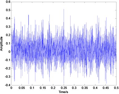
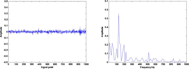
In order to verify the advantages of the proposed method in dictionary learning and random signal reconstruction, a simulation experiment is designed and carried out. The random signal is a random sparse signal of normal distribution generated by the function Sprandn(). Fig. 1 shows the generated random signal. Firstly, the random signals are used to carry out the dictionary learning and the sparse decomposition. The training matrix $Y$ is a matrix $m \times p$ of random generation in the experiment. In order to ensure the effectiveness of the dictionary learning, take $p = 5 m$ . The matrix with the size $m \times n$ generated by the random is used as the initial matrix $D$ , where $n = 2 m$ , and each column of the matrix is implemented the normalization process. In order to compare the performance of different methods in dictionary learning, the fixed iteration numbers (10 times) and the same sparsity ( $k =$ 15) are selected. The dictionary learning methods of ADMM and K-SVD are respectively carried out the dictionary learning, and record the learning time of the two methods. When the size of the dictionary is changed, the running speed of the two methods is compared.

Fig. 1Random signal generated by function Sprandn()

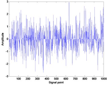
Fig. 2Compare of learning time in different dictionary size

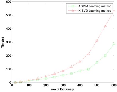
Fig. 2 shows the learning time of the dictionary row numbers from 50 to 600, the horizontal axis in Fig. 1 is the column numbers of the dictionary training, the vertical axis is the needed time of the learning process. The specific running time is given in Table 1. As shown in Fig. 2, it is clear that the running time of the ADMM dictionary learning is less than the K-SVD dictionary learning method in the same size of the testing matrix, dictionary and the iteration number. And with the increasing of the size of the dictionary, this advantage is more and more obvious. When the size of the dictionary is 600, the learning time of ADMM method is almost half of K-SVD method.

In order to further verify the superiority of the proposed method, the simulation signal is simulated as follows:

19

s (t) = 2 c o s (2 π f t + 5) + υ,

where $υ$ is the random noise of standard normal distribution, the signal-to-noise ratio is $S_{N R} =$ –10 dB. Fig. 3 shows the waveform of the simulation signal.

Table 1Specific time of dictionary learning

Size of dictionary	Learning time (s)
Size of dictionary	ADMM	K-SVD
50	3.25	5.72
100	12.44	17.40
200	31.33	45.74
300	55.23	87.08
400	87.00	156.8
500	150.56	310.81
600	289.34	530.23

Fig. 3The waveform of the simulation signal

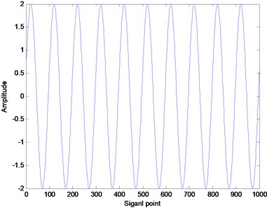
a) Original signal

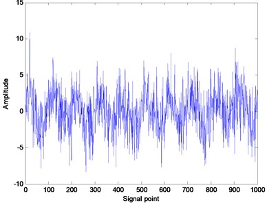
b) Signal with the noise

The training matrix $Y$ is obtained from the additive noise signal, and the dictionary is regarded as the initial dictionary. The original signal is decomposed by the sparse decomposition. The root mean square error (RMSE) of the reconstructed signal is obtained. The calculation formula of RMSE is as follows:

20

R M S E = \sqrt{‖I - I_{n}‖ {}_{F}^{2} / l e n g t h (I)},

where $I$ is the original signal, $I_{n}$ is the reconstructed signal. The size of the training matrix is 100×300, the size of the dictionary is 100×200, the sparsity of the decomposition is 15. The RMSE of the reconstructed signal with the change of the iteration number is shown in Fig. 4.

It can be seen from Fig. 4 that the RMSE of the reconstructed signal after dictionary learning is obviously less than the RMSE of without learning, and with the increase of iteration number in the dictionary learning, the RMSE of the reconstructed signal is gradually reduced. The RMSE of ADMM learning dictionary is obviously lower than the value of K-SVD dictionary learning, and with the increase of the numbers of iteration, the gap will continue to increase. But when the iteration number is more than 80, the value of RMSE tends to be stable, which indicates that the effect of signal decomposition is not increased with the increase of the iteration number of the dictionary learning. From the RMSE of the signal reconstruction, the ADMM dictionary learning algorithm is significantly better than the K-SVD dictionary learning.

Fig. 4RMSE of different methods

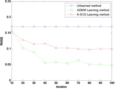
Fig. 5Time domain plot of inner race defect

5.2. Analysis of the bearing vibration signal for the fault feature extraction

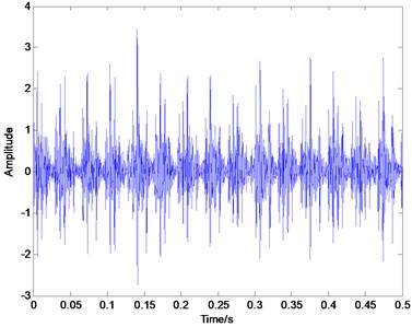
In order to verify the effectiveness of the proposed method in the sparse decomposition of bearing vibration signals, the actual experiment on fault identification of rolling element bearings is conducted in this paper. The vibration data of rolling bearings are provided by Case Western Reserve University (CWRU) [25]. The deep groove ball bearing with the type of 6205-2RS JEM SKF was used in the test. The vibration signals, when the rotating speed is 1797 rpm, and the sampling frequency is 12 KHz, are chosen to extract fault feature in this paper. The characteristic frequency of the inner race defect is calculated to be at 164 Hz, the outer race defect and the rolling element defect is 106 Hz and 128.9 Hz respectively based on the geometric parameters. Fig. 5, Fig. 6 and Fig. 7 illustrates the representative waveforms of the signal with the inner race defect, the outer race defect and the rolling element defect, respectively.

Fig. 6Time domain plot of outer race defect

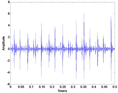
Fig. 7Time domain plot of rolling element defect signal

In this experiment, the data points of length 30000 are intercepted from the bearing vibration signal, which is used to construct the training matrix of 100×200, and the data points of length 1000 are intercepted from the remaining signal as the testing signal. The constructed dictionary is used as the dictionary to be learned, and the K-SVD and ADMM are used respectively to carry out the dictionary learning. According to the learned dictionary, the test signal is decomposed and reconstructed by using OMP algorithm, and the residual of the reconstructed signal is obtained, and the reconstructed signal is implemented by spectral analysis.

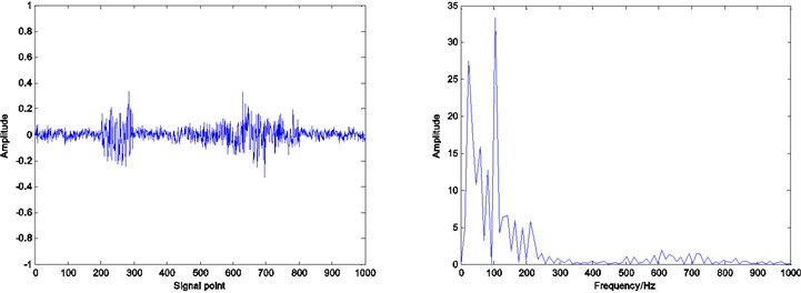
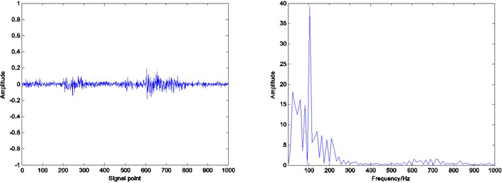
Fig. 8Residual and envelope spectrum by spare decomposition for inner race defect

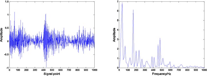
a) Without dictionary learning

b) K-SVD dictionary learning

c) ADMM dictionary learning

In the case of the same training matrix, the initial dictionary and the number of iterations, the dictionary learning and the sparse decomposition of test signals are implemented for obtaining the envelope spectrum of the reconstructed signal and the residual. When the iteration number of the dictionary learning is 30, the sparsity of decomposition is 20, Fig. 8, 9 and 10 show the envelope spectrum of the reconstructed signal and the residual results of the inner race defect, the outer race defect and the rolling element defect by using the related method.

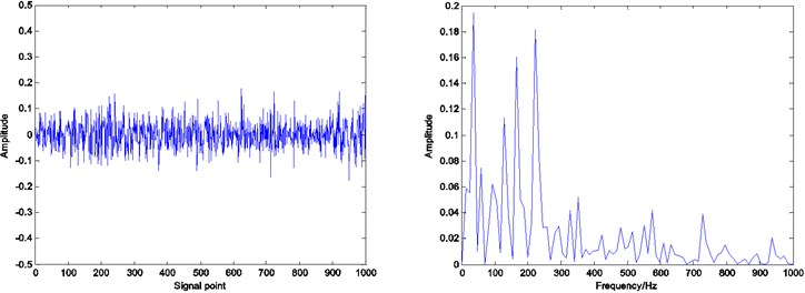
It can be seen that by Figs. 8, 9 and 10, under the same number of iterations and sparsity, the residual amount of reconstruction signal after the dictionary learning is far less than the residual amount of without learning. The residual amount of the proposed ADMM dictionary learning is smaller than that of the K-SVD dictionary learning method, which indicates that the dictionary constructed by ADMM dictionary learning is more consistent with the physical characteristics of the decomposed signal, and has better performance in sparse decomposition and reconstruction.

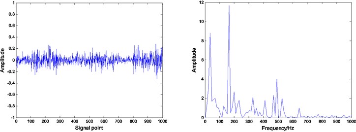
Fig. 9Residual and envelope spectrum by spare decomposition for outer race defect

a) Without dictionary learning

b) K-SVD dictionary learning

c) ADMM dictionary learning

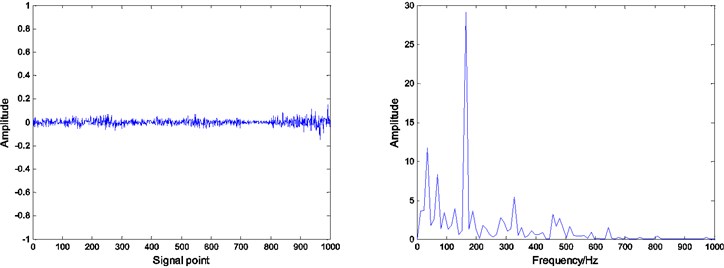
Compared with the envelope spectrum in Figs. 8, 9 and 10, it can be clearly seen that the decomposed effect of dictionary learning is better than that of the non-learning, and the fault frequency of the envelope spectrum is more obvious, and the interference frequency is less. At the same time, under the same condition, the resulting envelope spectrums of bearing fault signal obtained by ADMM dictionary learning and K-SVD dictionary learning are different. In the envelope spectrum of the bearing fault signal obtained by ADMM dictionary learning, the fault frequency of bearing inner race is very obvious. Although there are some interference frequencies, the amplitude is much smaller. However, the fault frequency can be identified in the envelope spectrum of the bearing fault signal obtained by K-SVD dictionary learning, but the amplitude of some interference frequencies is very high. It can be concluded that the dictionary obtained by ADMM dictionary learning is more consistent with the characteristics of the decomposed signal, and can get a better decomposition effect in the process of sparse decomposition.

Fig. 10Residual and envelope spectrum by spare decomposition for rolling element defect

a) Without dictionary learning

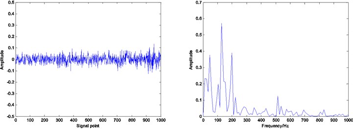
b) K-SVD dictionary learning

c) ADMM dictionary learning

6. Conclusions

In this paper, a dictionary learning method based on ADMM is presented for obtaining a better dictionary in structure, and the ADMM dictionary learning method combined with the orthogonal matching pursuit (OMP) is used to implement the sparse decomposition of the bearing vibration signal for the fault feature extraction. The experimental results show that this method has a faster speed and better sparse decomposition results. Compared with the K-SVD dictionary learning method, the proposed method has the superiority in the sparse decomposition of bearing signals. The experimental results show that, compared with the fixed dictionary and the K-SVD dictionary under the same conditions, the proposed ADMM dictionary learning method has not only fast learning speed, but also better reflect the characteristics of the decomposed signal. The proposed method is used to decompose the vibration signal of the rolling element bearing, the less residual can be obtained, the high frequency noise in the vibration signal of the rolling bearing can be effectively suppressed, and the fault characteristic frequency can be highlighted, which is very favorable for the fault diagnosis of the rolling element bearing.

References

Zhang X., Zhou J. Multi-fault diagnosis for rolling element bearings based on ensemble empirical mode decomposition and optimized support vector machines. Mechanical Systems and Signal Processing, Vol. 41, Issue 1, 2013, p. 127-140.

Publisher
Qu J., Zhang Z., Gong T. A novel intelligent method for mechanical fault diagnosis based on dual-tree complex wavelet packet transform and multiple classifier fusion. Neurocomputing, Vol. 171, 2016, p. 837-853.

Publisher
Sui W., Osman S., Wang W. An adaptive envelope spectrum technique for bearing fault detection. Measurement Science and Technology, Vol. 25, Issue 9, 2014, p. 095004.

Publisher
Jiang F., Zhu Z., Li W., et al. Robust condition monitoring and fault diagnosis of rolling element bearings using improved EEMD and statistical features. Measurement Science and Technology, Vol. 25, Issue 2, 2014, p. 025003.

Publisher
Lei Y., Lin J., He Z., et al. Application of an improved kurtogram method for fault diagnosis of rolling element bearings. Mechanical Systems and Signal Processing, Vol. 25, Issue 5, 2011, p. 1738-1749.

Publisher
Liu X., Bo L., He X., et al. Application of correlation matching for automatic bearing fault diagnosis. Journal of Sound and Vibration, Vol. 331, Issue 26, 2012, p. 5838-5852.

Publisher
Muruganatham B., Sanjith M. A., Krishnakumar B., et al. Roller element bearing fault diagnosis using singular spectrum analysis. Mechanical Systems and Signal Processing, Vol. 35, Issue 1, 2013, p. 150-166.

Publisher
Wang W., Lee H. An energy kurtosis demodulation technique for signal denoising and bearing fault detection. Measurement Science and Technology, Vol. 24, Issue 2, 2013, p. 025601.

Publisher
Mekhilef S. Numerical and experimental analysis of vibratory signals for rolling bearing fault diagnosis. Mechanics, Vol. 22, Issue 3, 2016, p. 217-224.

Publisher
Peng Z. K., Peter W. T, Chu F. L. A comparison study of improved Hilbert-Huang transform and wavelet transform: application to fault diagnosis for rolling bearing. Mechanical Systems and Signal Processing, Vol. 19, Issue 5, 2005, p. 974-988.

Publisher
Lei Y., Lin J., He Z., et al. A review on empirical mode decomposition in fault diagnosis of rotating machinery. Mechanical Systems and Signal Processing, Vol. 35, Issue 1, 2013, p. 108-126.

Publisher
Li Y., Xu M., Wei Y., et al. An improvement EMD method based on the optimized rational Hermite interpolation approach and its application to gear fault diagnosis. Measurement, Vol. 63, 2015, p. 330-345.

Publisher
Li Y., Xu M., Haiyang Z., et al. A new rotating machinery fault diagnosis method based on improved local mean decomposition. Digital Signal Processing, Vol. 46, 2015, p. 201-214.

Publisher
Cheng J., Yang Y., Yang Y. A rotating machinery fault diagnosis method based on local mean decomposition. Digital Signal Processing, Vol. 22, Issue 2, 2012, p. 356-366.

Publisher
Mallat S. G., Zhang Z. Matching pursuits with time-frequency dictionaries. IEEE Transactions on Signal Processing, Vol. 41, Issue 12, 1993, p. 3397-3415.

Publisher
He Q., Ding X. Sparse representation based on local time-frequency template matching for bearing transient fault feature extraction. Journal of Sound and Vibration, Vol. 370, 2016, p. 424-443.

Publisher
Ding X., He Q. Time-frequency manifold sparse reconstruction: a novel method for bearing fault feature extraction. Mechanical Systems and Signal Processing, Vol. 80, 2016, p. 392-413.

Publisher
Huang K., Aviyente S. Sparse representation for signal classification. Advances in Neural Information Processing Systems, 2006, p. 609-616.

Search CrossRef
Jafari M. G., Plumbley M. D. Fast dictionary learning for sparse representations of speech signals. IEEE Journal of Selected Topics in Signal Processing, Vol. 5, Issue 5, 2011, p. 1025-1031.

Publisher
Aharon M., Elad M., Bruckstein A. SVD: an algorithm for designing overcomplete dictionaries for sparse representation. IEEE Transactions on Signal Processing, Vol. 54, Issue 11, 2006, p. 4311-4322.

Publisher
Do T. H., Tabbone S., Terrades O. R. Sparse representation over learned dictionary for symbol recognition. Signal Processing, Vol. 125, 2016, p. 36-47.

Publisher
Pati Y. C., Rezaiifar R., Krishnaprasad P. S. Orthogonal matching pursuit: recursive function approximation with applications to wavelet decomposition. The 27th Asilomar Conference on Signals, Systems and Computers, 1993, p. 40-44.

Publisher
Boyd S., Parikh N., Chu E., et al. Distributed optimization and statistical learning via the alternating direction method of multipliers. Foundations and Trends in Machine Learning, Vol. 3, Issue 1, 2011, p. 1-122.

Publisher
Chen C., He B., Ye Y., et al. The direct extension of ADMM for multi-block convex minimization problems is not necessarily convergent. Mathematical Programming, Vol. 155, Issues 1-2, 2016, p. 57-79.

Publisher
http://csegroups.case.edu/bearingdatacenter.

Search CrossRef

Cited by

Fault Diagnosis of Rotating Equipment Bearing Based on EEMD and Improved Sparse Representation Algorithm

(2022)

A Parameter-Optimized Variational Mode Decomposition Investigation for Fault Feature Extraction of Rolling Element Bearings

(2021)

Dictionary learning technique enhances signal in LED-based photoacoustic imaging

(2020)

Research on Fault Feature Extraction Method of Rolling Bearing Based on NMD and Wavelet Threshold Denoising

(2018)

About this article

Received

14 August 2016

Accepted

08 November 2016

Published

31 December 2016

SUBJECTS

Fault diagnosis based on vibration signal analysis

DOI

https://doi.org/10.21595/jve.2016.17566

Keywords

sparse decomposition

alternating direction method of multipliers (ADMM)

dictionary learning

orthogonal matching pursuit (OMP)

K-SVD

rolling element bearing

fault feature extraction

Acknowledgements

This study was supported by State Key Laboratory of Alternate Electrical Power System with Renewable Energy Sources (Grant No. LAPS15019), the Fundamental Research Foundations for the Central Universities (Grant No. 2014JBZ017) and the National Science Foundation of China (Grant No. 51577007).

Author Contributions

Qingbin Tong, as the first author and corresponding author, his contribution is the idea of the article, writing and programming. Zhanlong Sun, his contribution is the preparation of article procedures, data analysis. Zhengwei Nie, his contribution is the preparation of article procedures, data analysis. Yuyi Lin, his contribution is to improve the language of the article. Junci Cao, his contribution is to further improve the article and the funding.

This is an open access article distributed under the Creative Commons Attribution License, which permits unrestricted use, distribution, and reproduction in any medium, provided the original work is properly cited.

Previous article in issue Previous Next article in issue Next

Research article

2024 01 21

Rolling bearing fault diagnosis based on variational mode decomposition and weighted multidimensional feature entropy fusion

Na Lei, Feihu Huang, Chunhui Li

Research article

2022 08 23

Repetitive impacts recovering using variational mode extraction with constructed reference enhanced by improved blind deconvolution

Wenliao Du, Xukun Hou, Hongchao Wang

Research article

2022 05 15

The enhancement of fault detection for rolling bearing via optimized VMD and TQWT based sparse code shrinkage

Xing Yuan, Huijie Zhang, Hui Liu

Research article

2021 11 26

Rolling bearing fault diagnosis with compressed signals based on hybrid compressive sensing

Zihan Chen

Q. Tong, Z. Sun, Z. Nie, Y. Lin, and J. Cao, “Sparse decomposition based on ADMM dictionary learning for fault feature extraction of rolling element bearing,” Journal of Vibroengineering, Vol. 18, No. 8, pp. 5204–5216, Dec. 2016, https://doi.org/10.21595/jve.2016.17566

Copy Extrica

Copied to clipboard!

TY  - JOUR
DO  - 10.21595/jve.2016.17566
UR  - https://doi.org/10.21595/jve.2016.17566
TI  - Sparse decomposition based on ADMM dictionary learning for fault feature extraction of rolling element bearing
T2  - Journal of Vibroengineering
AU  - Tong, Qingbin
AU  - Sun, Zhanlong
AU  - Nie, Zhengwei
AU  - Lin, Yuyi
AU  - Cao, Junci
PY  - 2016
DA  - 2016/12/31
PB  - JVE International Ltd.
SP  - 5204-5216
IS  - 8
VL  - 18
SN  - 1392-8716
ER  - 

Copy Ris

Copied to clipboard!

@article{Tong_2016,
	doi = {10.21595/jve.2016.17566},
	url = {https://doi.org/10.21595/jve.2016.17566},
	year = 2016,
	month = {dec},
	publisher = {{JVE} International Ltd.},
	volume = {18},
	number = {8},
	pages = {5204--5216},
	author = {Qingbin Tong and Zhanlong Sun and Zhengwei Nie and Yuyi Lin and Junci Cao},
	title = {Sparse decomposition based on {ADMM} dictionary learning for fault feature extraction of rolling element bearing},
	journal = {Journal of Vibroengineering}
}

Copy Bibtex

Copied to clipboard!

[1]Q. Tong, Z. Sun, Z. Nie, Y. Lin, and J. Cao, “Sparse decomposition based on ADMM dictionary learning for fault feature extraction of rolling element bearing,” Journal of Vibroengineering, vol. 18, no. 8, pp. 5204–5216, Dec. 2016, doi: 10.21595/jve.2016.17566.

Copy IEEE

Copied to clipboard!

Tong, Qingbin, Zhanlong Sun, Zhengwei Nie, Yuyi Lin, and Junci Cao. “Sparse Decomposition Based on ADMM Dictionary Learning for Fault Feature Extraction of Rolling Element Bearing.” Journal of Vibroengineering 18, no. 8 (December 31, 2016): 5204–16. https://doi.org/10.21595/jve.2016.17566.

Copy Chicago

Copied to clipboard!

Sparse decomposition based on ADMM dictionary learning for fault feature extraction of rolling element bearing

Abstract

1. Introduction

2. Sparse representation of signal

3. The basic principle of orthogonal matching pursuit

4. The proposed ADMM dictionary learning method

4.1. The alternating direction method of multipliers

4.2. ADMM dictionary learning method

5. Experimental analysis and discussion

5.1. Simulation analysis using proposed dictionary learning

5.2. Analysis of the bearing vibration signal for the fault feature extraction

6. Conclusions

References

Cited by

About this article

Related Articles