Radial basis approximation of single-phase flow in porous media based on the Green’s functions

1. Approximation of the steady-state fluid flow in porous media

Let us consider the problem of approximating solutions of differential equations describing two-dimensional fluid flow through a porous medium. To describe steady-state two-dimensional fluid flow we study the following boundary value problem:

with Neumann boundary condition ${\left.\partial P\left(\mathbf{r}\right)/\partial \mathbf{n}\right|}_{\mathrm{\Gamma }}=0\text{,}$ where $\mathrm{\lambda }\left(\mathbf{r}\right)=\mathbf{k}\left(\mathbf{r}\right)/\mu \text{,}$$\gamma =\rho g\text{,}$$\mathbf{r}\in \mathrm{\Omega }\subset {\stackrel{-}{\mathrm{\Omega }}}^2$; $P\left(\mathbf{r}\right)$ – pressure at point $\mathbf{r}=\left(x,y\right)\in \mathrm{\Omega }$; $\stackrel{-}{\mathrm{\Omega }}$ – computational domain with boundary $\mathrm{\Gamma }$; $\mathbf{n}$ – outer-pointing normal; $\mathbf{k}=\mathrm{d}\mathrm{i}\mathrm{a}\mathrm{g}\left(k_1,k_2\right)$ – diagonal tensor of absolute permeability; $h$ – reservoir thickness; $Z$ – reservoir depth; $\mu$ – fluid viscosity; $\rho$ – fluid density; $g$ – gravity acceleration; ${\mathbf{x}}_l$ – coordinates of $l$th well locations with flow rate $q_l$, $l=\overline{1,L}$; $L$ – number of wells; $\delta \left(\cdot \right)$ – generalized two-dimensional Dirac delta function.

Eq. (1) is Poisson’s equation with variable coefficients. For ordinary Poisson’s equation:

$\mathbf{r}=(x,y)\in D$, where $D$ denotes the entire plane, we can obtain the solution with Green’s function $G(\mathbf{r},\rho )$[1]:

where:

Such representation of solution to Eq. (2) in the presence of point sources and sinks is examined in [2], and it is known as well interference problem. Under constant coefficients and isotropy in Eq. (1) the solution Eq. (3) is given by:

where $q_l$ – well flow rate.

In case of variable coefficients Eq. (5) leads to significant errors in solution. We therefore propose the use of Green’s function Eq. (4) as radial basis functions $G\left(\left|\mathbf{r}-\rho \right|\right)$ to approximate Eq. (1) based on their linear combination. Coefficients of linear combination can be calculated through the numerical solution obtained by finite difference method. Let us consider rectangular domain $D=\left[a,b;c,d\right]$ which is divided into finite blocks $\mathrm{\Delta }x=b-a/n_x$, $\mathrm{\Delta }y=d-c/n_y$, where $n_x\times n_y$ – grid size.

Let us denote the numerical solution to Eq. (1) obtained by finite difference method as $P_{ij}$, $i=\overline{1,n_x}$; $j=\overline{1,n_y}$, and its approximation as $P_{ij}^a$, $i=\overline{1,n_x}$; $j=\overline{1,n_y}$. The approximation is constructed using linear combination of radial functions $G\left(\left|\mathbf{r}-\rho \right|\right)$. The radial function is undefined at a block contained source when $\mathbf{r}=\rho$. Therefore, its value at this point is set equal to a constant determined by the size of the block [3], e.g. $G_{ll}=-\mathrm{l}\mathrm{n}\left(\sqrt{\mathrm{\Delta }x\mathrm{\Delta }y}\right)/2\pi$.

Then the approximate expression can be written as:

where:

The sources can be with different signs. Here it is assumed that injection well is a source with positive sign and production well is a source with negative sign. We introduce also index $k$ which corresponds to the point $r_{ij}$, $i=\overline{1,n_x}$; $j=\overline{1,n_y}$; ${\alpha }_l$, ${\beta }_l$ – unknown coefficients that is determined through the condition $\sum _{k=1}^N{\left(P_k-P_k^a\right)}^2\to \underset{\alpha ,\beta }{\mathrm{m}\mathrm{i}\mathrm{n}}$, where $N=n_x{n}_y$.

To take into account Neumann boundary conditions Eq. (6) should be completed with additional image sources located outside of the computational domain. Each source $q_l$ is associated with four image sources $q_l^m$, $l=\overline{1,L}$; $m=\overline{\mathrm{1,4}}$. Their coordinates are given by:

thus we can rewrite Eq. (6) as:

We use the following notation:

where $\mathbf{d}$ – vector of known values; $\mathbf{X}$ – vector of unknown coefficients; $\mathbf{C}$ – calculated matrices. From $\mathbf{A}$, $\mathbf{B}$, $\mathbf{C}$ we construct block matrix:

Here $\mathbf{A}$, $\mathbf{B}$ are square matrices, $\mathbf{C}$, $\mathbf{G}$ are rectangular matrices ($N>2L$).

According to the minimum condition of standard deviation we obtain matrix equation:

We multiply Eq. (8) from left by the transposed matrix ${\mathbf{G}}^T$: ${\mathbf{G}}^T\mathbf{G}\mathbf{X}={\mathbf{G}}^T\mathbf{d}$.

Then we calculate inverse of the matrix ${\mathbf{G}}^T\mathbf{G}$ and obtain expression to find unknown coefficients:

The operation ${\left({\mathbf{G}}^T\mathbf{G}\right)}^{-1}{\mathbf{G}}^T={\mathbf{G}}^{+}$ is called pseudoinversion [4], and the approximation based on radial basis function is known as radial basis neural network.

Then radial approximation appears as follows:

Coefficients $\mathbf{X}$ are calculated for some preselected source locations and their flow rates. Then the approximation Eq. (10) is used for arbitrary source locations and their flow rates. The number of sources should be less than or equal to $L$. For a smaller number of sources, the flow rates of extra sources are set to zero. According to the Neumann boundary condition the material balance that accounts for source terms should be zero [5, 6].

For illustration, let us consider the following case study. The domain $D=\left[a,b;c,d\right]$, $a=$0; $b=$1000 m; $c=$0; $d=$1000 m was divided into 256×256 blocks of finite difference grid. Reservoir thickness was changed according to $h\left(\mathbf{r}\right)=10(1+0.1\mathrm{s}\mathrm{i}\mathrm{n}(4\pi (x+y)\left)\right)\text{,}$ fluid mobility was changed according to $\lambda \left(\mathbf{r}\right)=10^{-9}\left(1+0.2\mathrm{s}\mathrm{i}\mathrm{n}\left(2\pi x\right)+0.15\mathrm{c}\mathrm{o}\mathrm{s}\left(2\pi y\right)\right)$. There were 10 wells (5 production wells and 5 injection wells) in the domain. The absolute values of flow rates of all sources were the same and equal to $Q=\mathrm{}$50 m³/s. The sources were randomly located in the domain. To calculate pressure in blocks multigrid method with 7 nested grids was used.

Fig. 1 demonstrates distribution of the normalized pressure $p=(P-P^{\mathrm{m}\mathrm{i}\mathrm{n}})/(P^{\mathrm{m}\mathrm{a}\mathrm{x}}-P^{\mathrm{m}\mathrm{i}\mathrm{n}})$ in the domain, where $P^{\mathrm{m}\mathrm{a}\mathrm{x}}$, $P^{\mathrm{m}\mathrm{i}\mathrm{n}}$ – maximum and minimum pressure values. The distribution of the approximate pressure is shown in Fig. 2.

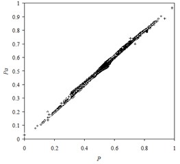
As shown in Fig. 3, comparison of the pressure values in midsection of the domain demonstrates relatively sufficient approximation.

Then we changed locations of the sources and their flow rates in random manner. Comparison of the numerical pressure values with their approximate values in midsection of the domain for different source distribution is shown in Fig. 4.

As can be seen, the radial network is well trained and provides sufficient approximation of the data that is independent of the training set. Fig. 5 demonstrates comparison of the numerical pressure values with their approximate values for all blocks of the domain.

The standard deviation of the approximate pressure values from their numerical values is 0.95 %. The plus signs in Fig. 5 depict pressure values in blocks contained sources. The maximum deviations are observed in these particular blocks where pressure changes more rapidly. The results show that the Neumann boundary conditions are satisfied. It should be noted that Neumann boundary conditions are the most difficult case study especially when they are applied for the entire boundary.

Fig. 1Pressure distribution obtained by finite difference method

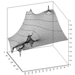
Fig. 2Approximate pressure distribution

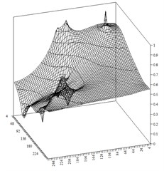
Fig. 3Comparison of the numerical pressure values with their approximate values in midsection of the domain

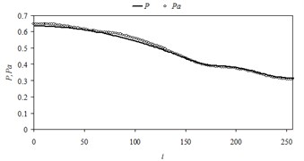
Fig. 4Comparison of the numerical pressure values with their approximate values in midsection of the domain in case of different source locations

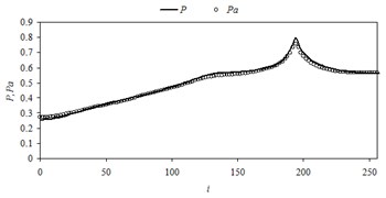
Fig. 5Comparison of the numerical pressure values with their approximate values for all blocks of the domain

2. Approximation of the nonstationary fluid flow in porous media

For the case of compressible fluid flow and rock porosity depending on the pressure Eq. (1) becomes parabolic differential equation:

where $\lambda \left(\mathbf{r}\right)=\mathbf{k}\left(\mathbf{r}\right)/\mu B\text{;}$$\beta \left(\mathbf{x}\right)=\phi \left(\mathbf{r}\right)c_{\mathcal{l}}/B°+\phi °\left(\mathbf{r}\right)c_{\phi }/B\text{;}$$\rho =\rho °\left(1+c_{\mathcal{l}}\left(P-P°\right)\right)\text{,}$$B=B°/1+c_{\mathcal{l}}\left(P-P°\right)\text{,}$$\mu =\mu °/1-c_{\mu }\left(P-P°\right)\text{,}$$\phi \left(\mathbf{r}\right)=\phi °\left(\mathbf{r}\right)\left(1+c_{\phi }\left(P-P°\right)\right)$, $\phi \left(\mathbf{r}\right)$ – rock porosity; $B$ – fluid formation volume factor; $P°$ – reference pressure. Eq. (11) is complemented by the initial condition:

For parabolic model equation:

there is Green’s function solution as well [1]:

where $G(t,\mathbf{r};\tau ,\xi )$ – Green’s function, which can be constructed from eigenfunctions ${\psi }_k$ and eigenvalues ${\lambda }_k$ of Helmholtz equation:

Eq. (14) and Eq. (15) can be used as a basis for approximate solution to Eq. (11). It is important to note that Green’s function (15) can be represented as product of two functions (separation of variables): the first one depends exponentially only on time variable, the second one depends only on spatial variables.

Assume first that flow rate of sources is time-independent. Let us restrict ourselves to the one summand in Eq. (15). Then Eq. (15) can be rewritten as:

where $\mathrm{\Psi }(\xi ,\mathbf{r})$ – some function sought for approximation.

Time integration of Eq. (14) gives:

It follows from Eq. (16) that solution to nonstationary equation Eq. (13) contains steady-state component:

To which solution Eq. (16) converges asymptotically as $t\to \mathrm{\infty }$. The second term $e^{-\lambda t/{\alpha }^2}\underset{V}{\int }\mathrm{\Psi }(\xi ,\mathbf{r}){\mathrm{\Phi }}_0\left(\xi \right)dV\left(\xi \right)$ corresponds to the initial condition as $t\to 0$. Therefore, approximation problem is solved in two steps. At first we seek an approximant to a steady-state solution as $t\to \mathrm{\infty }$. For this purpose the radial function Eq. (7) denoted as $G_S(\xi ,\mathbf{r})$ is used. For the second term in Eq. (16) we take unit integral transform to satisfy the given initial condition. Then the parameter nonstationarity $\lambda$ is adjusted. For best approximation on time several terms of series can be used in Eq. (15), so Green’s function can be presented as:

and solution Eq. (16) can be written as:

It should be noted that the underlying considerations are not strictly mathematically sound and needed only to choose basis functions when constructing the approximant.

Let us consider the case where $\sum _{l=1}^{L}h\left({\mathbf{r}}_l\right)q_l=\delta q\ne 0$. The steady-state solution to Eq. (11) as $\partial P/\partial t\to 0$ doesn’t exist subject to the Neumann boundary condition. To construct function $G_S(\xi ,\mathbf{r})$ we introduce background sources:

for each grid blocks of the computational domain. Now we can define the corresponding steady state and fit the function $G_S(\xi ,\mathbf{r})$ which describes this state. Eq. (17) is now as follows:

If the flow rate of a source is a function of time $f(t,\mathbf{r})$ then the nonstationary process is divided into time steps of length $\mathrm{\Delta }{t}^n$ by analogy with finite-difference representation, so the approximate expression for pressure is written as:

where ${\alpha }^2=h\left(\mathbf{r}\right)\beta \left(\mathbf{r}\right)$; $f(t,{\mathbf{r}}_l)=h\left(\mathbf{r}\right)\sum _{l=1}^L{q}_l\left(t\right)\delta \left(\mathbf{r}-{\mathbf{r}}_l\right)$.

For one summand in sum Eq. (18) can be written in the form:

According to the condition $\sum _{i,j,n}{\left(P^a(t^n,r_{ij})-P(t^n,r_{ij})\right)}^2\to \underset{\lambda }{\mathrm{m}\mathrm{i}\mathrm{n}}$ we obtain the expression for coefficient $\lambda$ based on the calculation of $P_{ij}^n$ by finite-difference method:

where $P_{ij}^n$ – calculated pressure values; $N$ – number of time steps. The results showed that in most practical cases $\lambda \approx \text{0.25}$.

Let us consider the case study under the same conditions as in the steady-state case. In addition, we assumed that porosity $\phi °=0.15$, and coefficients $c_{\phi }=\mathrm{}$10^-4; $c_l=$2∙10^-4; $c_{\mu }=\mathrm{}$0. The stationary function $G_S(\mathrm{\rho },\mathbf{r})$ was taken as a result of previous training. The material unbalance was $Q=\mathrm{}$39 m³/s. The calculated value of $\lambda$ was $\lambda =\text{0.27}$. Fig. 6 compares numerical and approximate pressures for different time steps in midsection of the domain.

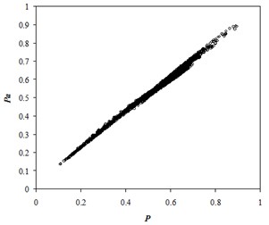
The solid lines correspond to pressure obtained numerically by finite-difference method, and the circles correspond to approximate pressure. The comparison of the normalized numerical and approximate pressure values for all the grid blocks is shown in Fig. 7.

The standard deviation of the approximate pressure values from their numerical values is 1.84 %, that is approximately twice as high as for steady-state flow.

Fig. 6The comparison of the numerical and approximate pressures in midsection of the domain in case of nonstationary flow 1 – t-=0.2; 2 – t-=0.4; 3 – t-=0.6; 4 – t-=0.8

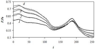
Fig. 7Comparison of the normalized numerical and approximate pressures

3. Conclusions

1) The developed model of radial approximation of the steady-state equation of the fluid flow in porous media based on basis Green’s functions provides that standard deviation of the approximate pressure from its numerical values will be within the range 0.95-1.05 %. Such basis functions are used to approximate solution of the nonstationary multiphase flow in porous media as well.

2) To approximate solution of the nonstationary fluid flow in porous media Green’s function is used. It is represented as a product of two terms (separation of variables): the first one exponentially depends only on time; the second one depends only on spatial coordinates. The use of background sources allows the construction of approximants which are applicable for time-varying flow rates of the sources and unbalanced flow rates.

References

-
Korn G. A., Korn T. M. Mathematical Handbook for Scientists and Engineers; Definitions, Theorems, and Formulas for Reference and Review. McGraw-Hill, New York, 1968, p. 1151.
Basniev K. S., Kochina I. N., Maksimov V. M. Underground Hydrodynamics. Nedra, Moscow, 1993, p. 416, (in Russian).
Kanevskaya R. D. Mathematical modeling of hydrodynamic processes of hydrocarbon deposit development. Izhevsk, 2003, p. 128, (in Russian).
Osowski S. Neural Networks for Information Processing. Finance and Statistics, Moscow, 2002, p. 344, (in Russian).
Chanson H. Applied Hydrodynamics: An Introduction to Ideal and Real Fluid Flows. CRC Press, Taylor & Francis Group, Leiden, The Netherlands, 2009, p. 478.
Economides Michael J., Nolte Kenneth G. Reservoir Stimulation. Wiley, USA, 2000, p. 856.
About this article