Abstract
Most engineering structures include nonlinearities. In some cases, the nonlinearity may cause little effect and can be ignored, thus, the system can be seen as linear and analyzed by linear theory. However, sometimes the nonlinear effects are big enough, not be ignored. It is very important to successfully detect, localize and parametrically identify nonlinearity in such cases. The describing function method can identify the structural nonlinearity by the frequency response function measured under a harmonic excitation. In this paper, the theory of using describing function method to identify structural nonlinearity is introduced. A case study using describing function method to identify a MDOF nonlinear system with two nonlinear elements at different locations is given to demonstrate the application of this method.
1. Introduction
Engineering structures generally exhibit nonlinearities. Sometimes it may lead to some unpredictable and undesirable consequence. Identification of nonlinearities becomes more and more important. In the past decades, many researchers have focused on the identification of nonlinearities in multi degree of freedom (MDOF) system. Studies in this field can be classified in two groups: time domain and frequency domain techniques. Time domain techniques use time as the independent variables and generally focus on time series [1]. Frequency domain techniques transform the time domain signal into frequency domain and first order or higher order harmonic responses are used to localize and/or identify nonlinearity in structures. Some methods use broad band random signals.
A lot of work has been done in frequency domain methods for identification of nonlinear MDOF systems. He and Worden proposed the frequency response function, FRF, method [2], it uses the response that we get from the system under a series of sinusoidal signals excitation with increasing frequencies to identify the nonlinear system. Similar to the FRF, the multi-harmonic FRF method can be used to identify a system through the responses [3]. Based on the definitions of the frequency response function and the first-order harmonic balance method, Özgüven and Tanrikulu proposed the method analyzing the nonlinear structures using the describing functions [4]. Then Özer and Özgüven introduced non-linearity numbers that can be obtained from harmonic vibration measurements [5], in order to localize any non-linear element in the system. A further research was made by Özer and Özgüven [6]. Based on the previous studies they proposed an approach to calculate the describing function’s approximate solutions by using the Sherman-Morrison Method. Arslan and Aykan proposed a method to make a modal model of a nonlinear structure from measured frequency responses [7]. Aykan and Özgüven introduced a method to calculate the entire linear FRF matrix from only one row of the matrix and then proposed a method to transform the describing function into the restoring force to make it more visualized [8].
The theory of using describing function method to identify structural nonlinearity is given below in detail. A case study is given to demonstrate the application of this method in a MDOF system with more than one nonlinearity at different locations.
2. Theory
The equation of motion for a nonlinear MDOF system under excitation can be written as:
where , , and are mass, viscous damping and stiffness matrices of the linear system, respectively. and stand for the external force and the response of the system. represents the nonlinear internal force in the system, and it is a function of the displacement and/or velocity response of the system, depending on the type of nonlinearity present in the system.
A harmonic excitation with circular frequency may be written:
Using first order harmonic balance method, the response is assumed to consist of only the first fundamental harmonic, disregarding higher order harmonics:
Since the response is assumed to be harmonic, the internal nonlinear forces can be assumed to be harmonic too, which can be written as [6]:
where is response dependent ‘non-linearity matrix’. The ‘non-linearity matrix’ can be formed by using describing function representations of internal non-linear forces as follows:
where is the describing function of nonlinearity between th and th DOFs. Since using fundamental harmonic component of nonlinear force between th and th DOFs, can be evaluated by [4]:
where is the nonlinear force between th and th DOFs and is the amplitude of the relative displacement of th and th DOFs. At this point, linearization via describing function is equivalent to linearization using first order harmonic balance method.
Nonlinear forces in the system can be expressed in a matrix form. This representation has been first presented by Budak and Özgüven [9] and then the method is generalized for any type of nonlinearity by Tanrikulu et al. [4] by using describing functions.
From the equations above the equation of motion of a nonlinear system can be written as:
Then the nonlinear frequency response function (FRF) matrix can be calculated as:
The FRF of underlying linear system, , can be written as:
Notice that at different excitation levels the nonlinear FRF may be different due to the non-linearity matrix. The non-linearity matrix can formally be obtained by:
It should be pointed out that Eq. (11) will not work in general to calculate the non-linearity matrix, as the columns of , corresponding to force input at different DOFs, will be measured with different amplitudes at the DOFs with nonlinearities. For systems with many nonlinear elements it may be impossible to keep the amplitudes in question constant for different force inputs. This means that the non-linear FRF matrix isn’t consistent. Eq. (11) may anyway be used to get a hint of the position and nature of the nonlinear elements, see example below.
To avoid the problem, a method to use only one force input, only one column, in is shown here. Post-multiplying both sides in Eq. (11) by yields:
The non-linearity numbers [5] then can be obtained to localize any non-linear element in the system. From the th column of Eq. (12) we can get:
where is the th column of unit matrix .Then the th row of Eq. (13) can be written as:
And the “non-linearity number (NLN)” for row can be defined as:
In Eq. (15), any nonlinearity connected to DOF may lead to nonzero element of , then the may tell if there is a nonlinear element connected to DOF . The can be obtained from the right side of Eq. (14):
is dependent on the frequency and amplitude of the applied force, therefore will have different values at different excitation frequencies and amplitudes. It is advisable to use the sum of for different excitations to find out the nonlinear element location.
After localization of structural non-linearity, the nonlinear parameter(s) could be calculated. Eq. (11) cannot generally be used to calculate the describing function in order to determine the nonlinear type and parameter. Eq. (15) and (16) can be used instead. As is shown in example below, after the use of Eq. (11) and (16), one can make a guess on non-linearity matrix . Then, using Eq. (15) and (16) for different frequencies and/or force amplitudes, the describing function as function of response amplitude can be estimated. The form and parameter values may then be estimated with curve fitting methods. This also works for MDOF systems with multiple nonlinearities in different DOFs.
3. Case study
A four degree of freedom system with two nonlinear elements is studied.
Fig. 1System used for case study
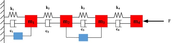
System parameters are: N s/m, N s/m, N s/m, N s/m, N/m, N/m, N/m, N/m, kg, kg, kg, kg.
The nonlinear element from m1 to ground is “square with sign”, with nonlinear force, , and describing function :
The nonlinear element connecting and is a cubic spring with and :
The linear FRF is calculated from the linear system, The FRF around the first resonance is calculated with swept sine input for six force amplitudes, 0.005 N and 0.1-0.5 N with step 0.1 N, as shown in Fig. 2.
Fig. 2Linear and Nonlinear FRF H14
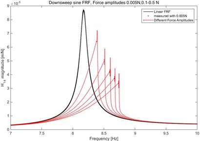
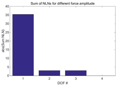
Fig. 3Sum of NLN of different amplitude
It can be seen that the FRF at force amplitude 0.005 N can be used as linear FRF and 9 Hz is a good choice for simulation from Fig. 2. The complete linear and nonlinear FRF matrices, and , are calculated in a simulation with sinusoidal input force, frequency 9 Hz, amplitude 0.005N and 0.2 N, respectively. The simulation is performed with functions in a nonlinear MATLAB toolbox [10].
The sampling frequency is set to 163.84 Hz, 8192×0.02, which with an analysis FFT block size of 8192 gives 0.02 and a clean sine response for 9 Hz at frequency point 451. The force signal has a length of 16384 samples, and the analysis is performed on the last 8192 samples, where the response has reached a stable value.
The result for :
1.0e+004*;
2.1581+0.1553i, 0.6122+0.0195i, 0.2159+0.0026i, –0.6797–0.0876i;
–0.2880-0.0152i, 0.5001+0.0277i, –0.2667-0.0165i, 0.0132+0.0032i;
0.2880+0.0152i, –0.5001-0.0277i, 0.2667+0.0165i, –0.0132-0.0032i;
0.0000-0.0000i, –0.0000+0.0000i, 0.0000-0.0000i, –0.0000+0.0000i.
The structure of is not correct. But it contains some information about the nonlinear elements present. Rows 2 and 3 have the same look with opposite sign. That suggests there is a nonlinear element connected between and . Row 1 is nonzero and unique suggesting another nonlinear element connected from to ground. Row 4 is basically zero, indicating has no nonlinear element connected. This assumption may be confirmed by calculation of the NLNs. We use the method with only one force input described above. We input the force with frequency 9 Hz at , and vary the force amplitude between 0.1 to 0.8 N in 70 steps. For each step we measure column 4 in the nonlinear FRF matrix and the amplitudes of , and . The NLN result is shown in Fig. 3. From this we may draw the conclusion that m1 is connected to ground with one nonlinear element, as NLN for DOFs 1 is unique. NLN for DOFs 2 and 3 have the same absolute value, leading us to assume that m2 and m3 are connected with another nonlinear element. NLN for DOF 4 is close to zero, telling us that m4 has no nonlinear element connected.
We can then assume the matrix to be:
For each force amplitude step we calculate estimates of and using Eq. (15) and Eq. (16). The results are plotted as functions of the measured response amplitudes. The theoretical describing functions are plotted in the diagrams for reference, and the agreement is quite good.
Fig. 4Estimated DF for x1*absx1 nonlinearity
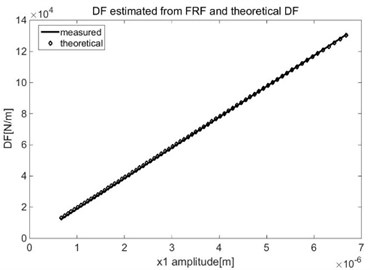
Fig. 5Estimated DF for cubic nonlinearity
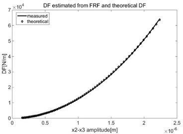
A polynomial fit to gives the coefficient 2.296e+010. A polynomial fit to gives the coefficient 1.696e16.
4. Conclusions
From the case study, the possibility to identify the nonlinearities in a MDOF nonlinear system with more than one nonlinear element at different locations by using describing function method is shown. If the linear FRF matrix may be obtained this method, it can be used with only column of the nonlinear FRF matrix. This method makes it possible to identify nonlinearity type because the describing function curve for each type is unique.
References
-
Chen Q., Tomlinson G. R. A new type of time series model for the identification of non-linear dynamical systems. Mechanical Systems and Signal Processing, Vol. 8, Issue 5, 1994, p. 531-549.
-
He J., Ewins D. J. A simple method of interpretation for the modal analysis of nonlinear systems. International Modal Analysis Conference, 1987, p. 626-634.
-
Storer D. M., Tomlinson G. R. Recent developments in the measurement and interpretation of higher order transfer functions from non-linear structures. Mechanical Systems and Signal Processing, Vol. 7, Issue 2, 1993, p. 173-189.
-
Tanrikulu O., Kuran B., Özgüven H. N. Forced harmonic response analysis of nonlinear structures using describing functions. AIAA Journal, Vol. 31, Issue 7, 1993, p. 1313-1320.
-
Özer M. B., Özgüven H. N. A new method for localization and identification of non-linearities in structures. Biennial Conference on Engineering Systems Design and Analysis, 2002.
-
Özer M. B., Özgüven H. N., Royston T. J. Identification of structural nonlinearities using describing functions and Sherman-Morrison method. Mechanical Systems and Signal Processing, Vol. 23, Issue 1, 2009, p. 30-44.
-
Arslan Ö., Aykan M., Özgüven H. N. Parametric identification of structural nonlinearities from measured frequency response data. Mechanical Systems and Signal Processing, Vol. 25, Issue 4, 2011, p. 1112-1125.
-
Aykan M., Özgüven H. N. Parametric identification of nonlinearity in structural systems using describing function inversion. Mechanical Systems and Signal Processing, Vol. 40, Issue 1, 2013, p. 356-376.
-
Budak E., Özgüven H. N. A method for harmonic response of structures with symmetrical non-linearities. International Seminar on Modal Analysis and Structural Dynamics, 1990.
-
Ahlin K. Toolbox for simulation and parameter identification of nonlinear mechanical systems. Proceedings of IMAC 25, 2007.
About this article
