Feature extraction and fault diagnosis of wind power generator vibration signals based on empirical wavelet transform

Chen, Xuejun; Yang, Yongming; Yang, Ning

doi:10.21595/jve.2017.17374

Journal of Vibroengineering

Browse Journal

Submit article

Published: 15 May 2017

Check for updates

Feature extraction and fault diagnosis of wind power generator vibration signals based on empirical wavelet transform

Xuejun Chen¹

Yongming Yang²

Ning Yang³

¹Department of Mechanical and Electrical Engineering, Putian University, Putian, 351100, China

^{2, 3}State Key Laboratory of Power Transmission Equipment and System Security and New Technology, Chongqing University, Chongqing, 400044, China

Corresponding Author:

Xuejun Chen

Cite the article Download PDF

Downloads 1380

WoS Core Citations 2

CrossRef Citations 2

Abstract

Given the nonlinear and nonstationary characteristics of wind power generator vibration signals, the empirical wavelet transform (EWT)-based method is proposed to analyze the vibration signal characteristics and to diagnose faults. The adaptive Fourier spectrum segmentation of EWT is analyzed, and an appropriate wavelet filter is constructed to extract different AM-FM mode functions. The Hilbert transform is conducted, and the signal modal component energy is normalized to obtain vibration feature quantities. A probabilistic neural network (PNN) is used to perform the classification and diagnosis of wind power generator vibration faults. The experiments are constructed based on simulation signals and vibration signals before the proposed method and Hilbert-Huang transform (HHT) are used to perform mode decomposition and to analyze the time-frequency energy spectrum. The experimental results showed that the obtained resolution modes by EWT are within the corresponding time domain signal characteristics. The number of mode decomposition layers is less than that of empirical mode decomposition. No characteristics of false modal are observed. The time-frequency energy spectrum diagram can better reflect the characteristics of original vibration signal than the spectrum based on HHT. The PNN-based vibration fault judgment can achieve an accuracy rate of 90 % with limited training samples.

1. Introduction

As a green renewable energy, wind energy has been developed and used by more countries. Wind power is also expected to dominate energy structure adjustment in the future. Therefore, wind power equipment rapidly developed. The normal operation of wind power generators can directly affect the safety and economic benefits of power grids. Therefore, technologies for power generator condition monitoring and for fault diagnosis urgently need to be developed [1, 2]. Wind power generator vibration monitoring is a method for evaluating the condition of power generator as well as the early detection and tracking of wind power generator failure [3-6].

With the development of digital signal processing, time-frequency analysis methods have made remarkable achievements. Wigner-Ville distribution solves the existing problems of short-time Fourier transform to some extent; this approach has high-frequency resolution, energy concentration, and other characteristics, thereby making it suitable for nonstationary signal processing and analysis. However, the Wigner-Ville distribution has cross terms and other problems in multi-component signal [7, 8]. Wavelet analysis has multi-resolution features and the ability to characterize local signal characteristics, but it has several problems in basis function selection, sensitive parameters, and the failure of accurately describing the frequency with time conversion; when analyzing fault information, aliasing phenomenon and difficulty in judging singularities may occur [9-11]. Blind source separation can restore source signals by observing the signal output recognition system, with good effects in extracting the characteristics of weak signal sources; this approach has good de-noising effects, but the theory and algorithm have the shortcomings of nonlinear mixtures and the changing number of signal sources [12-14].

Given the nonlinear nonstationary signals, Huang proposed the Hilbert-Huang transform (HHT), which first performed adaptive empirical mode decomposition (EMD) of signals followed by Hilbert transform to obtain Hilbert spectrum and time–frequency energy spectrum, as well as analyzed the signal frequency localization [15]. However, the EMD method may produce modal aliasing and envelope fitting error for some signal decomposition results, thereby causing new problems for the analysis and interpretation of some signals [16, 17]. Gilles combined the advantages of adaptive empirical mode decomposition and wavelet analysis theory to propose the empirical wavelet transform (EWT), which is a major breakthrough in nonstationary signal processing [18]. The core idea of EWT is to perform adaptive segmentation based on the Fourier spectrum characteristics of signals, to construct proper wavelet filters for extracting different AM-FM components, to conduct Hilbert transform of AM–FM decomposition mode, and to obtain the instantaneous frequency and amplitude. EWT adaptive mode decomposition is superior to EMD because it has smaller calculation volume than the EMD method, avoids modal aliasing, and has strong robustness.

Some researchers used EWT as a novel signal processing analysis tool and applied it to research on nonstationary signals, with good results [19-21]. The wind power generator vibration signal is a typical nonlinear and nonstationary signal because EWT can achieve adaptive decomposition of the nonstationary signal and have higher time–frequency resolution. Therefore, this paper proposes that EWT should be used to conduct exploratory feature analysis of wind power generator vibration signals and to diagnose wind power generator vibration fault based on a probabilistic neural network (PNN), thereby providing a new method for the monitoring and analysis of wind power generator safety production and fault diagnosis based on vibration signals.

2. EWT-based on vibration signal analysis

2.1. EWT method

The essence of EMD is to decompose the original signal $f (t)$ into $N$ intrinsic mode function (IMF) components $c_{i} (t)$ and the sum of the remainder $r_{n} (t)$ , as shown in Eq. (1):

1

f (t) = \sum_{i = 1}^{N} c_{i} (t) + r_{n} (t) .

The decomposition method has a screening iteration termination condition, end effects, modal aliasing, and other problems. To overcome its shortcomings, Gilles combined wavelet analysis based on EMD method and presented EWT. This approach decomposes the original signal $f (t)$ into the $N +$ 1 mode function $f_{i} (t)$ , that is:

2

f (t) = \sum_{i = 0}^{N} f_{i} (t) .

The $f_{i} (t)$ in Eq. (2) is defined as an AM-FM signal, as shown in Eq. (3):

3

f_{i} (t) = F_{i} (t) c o s (ϕ_{i} (t)) .

In Eq. (3), $F_{i} (t) > 0$ and $ϕ_{i}^{'} (t) > 0$ by assuming that the changes in $F_{i}$ and $ϕ_{i}^{'}$ are much slower than those in $ϕ_{i}$ . This method is based on wavelet analysis. The method conducts adaptive segments according to the signal’s Fourier spectral characteristics and establishes a suitable wavelet filter to extract different AM-FM components. By assuming that the Fourier support [0, $π$ ] is divided into $N$ consecutive sections $Λ_{n}$ ; $ω_{n}$ is defined as the boundary of successive sections, and the midpoint between the two maxima adjacent to the signal Fourier spectrum is taken and expressed as Eq. (4):

4

\{\begin{array}{l} Λ_{n} = [ω_{n - 1}, ω_{n}], n = 1,2, \dots, N, (ω_{0} = 0, ω_{N} = π), \\ ⋃_{n - 1}^{N} Λ_{n} = [0, π] . \begin{array}{l} \begin{array}{l} \begin{array}{l} \begin{array}{l}  \end{array} \end{array} \end{array} \end{array} \end{array}

Eq. (4) takes each $ω_{n}$ as the center; the width $T_{n} = 2 τ_{n}$ is taken as the transition section, as shown in Fig. 1.

Fig. 1Fourier shaft split

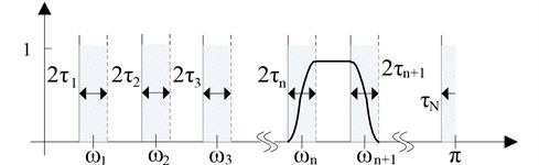
An empirical wavelet is defined as the band-pass filter on each $Λ_{n}$ . The empirical wavelet is constructed according to the Meyer wavelet, thereby determining the empirical scaling function and empirical wavelet function, which are shown as Eq. (5) and (6) [18]:

5

{\hat{ϕ}}_{n} (ω) = \{\begin{array}{l} 1, & |ω| \leq ω_{n} - τ_{n}, \\ c o s [\frac{π}{2} β (\frac{1}{2 τ_{n}} (|ω| - ω_{n} + τ_{n}))], & ω_{n} - τ_{n} \leq |ω| \leq ω_{n} + τ_{n}, \\ 0, & other, \end{array}

6

{\hat{ψ}}_{n} (ω) = \{\begin{array}{l} 1, & ω_{n} + τ_{n} \leq |ω| \leq ω_{n + 1} - τ_{n + 1}, \\ c o s [\frac{π}{2} β (\frac{1}{2 τ_{n + 1}} (|ω| - ω_{n + 1} + τ_{n + 1}))], & ω_{n + 1} - τ_{n + 1} \leq |ω| ω_{n + 1} + τ_{n + 1}, \\ s i n [\frac{π}{2} β (\frac{1}{2 τ_{n}} (|ω| - ω_{n} + τ_{n}))], & ω_{n} - τ_{n} \leq |ω| \leq ω_{n} + τ_{n} \\ 0, & other . \end{array}

The $τ_{n}$ and $β (x)$ in Eq. (5) and Eq. (6) can be expressed as follows:

7

\{\begin{array}{l} τ_{n} = γ ω_{n}, 0 < γ < 1, γ < m i n_{n} (\frac{ω_{n + 1} - ω_{n}}{ω_{n + 1} + ω_{n}}), \\ β (x) = x^{4} (35 - 84 x + 70 x^{2} - 20 x^{3}) . \end{array}

Similar to traditional wavelet transform, EWT is defined as $W_{f}^{ε} (n, t) .$ $F F T (\cdot)$ and $I F F T^{- 1} (\cdot)$ are used to represent Fourier transform and Fourier inverse transform, and then the EWT detail coefficient is calculated according to the inner product of signal and empirical wavelet function:

8

W_{f}^{ε} (n, t) = 〈f, ψ_{n}〉 = \int f (τ) \bar{ψ_{n} (τ - t)} d τ = I F F T^{- 1} (f (ω) {\hat{ψ}}_{n} (ω)) .

$W_{f}^{ε} (0, t)$ is used to represent the approximate coefficient, and it can be generated by the inner product of signal and empirical scaling function:

9

W_{f}^{ε} (0, t) = 〈f, ϕ_{1}〉 = \int f (τ) \bar{ϕ_{1} (τ - t)} d τ = I F F T^{- 1} (f (ω) {\hat{ϕ}}_{1} (ω)) .

${\hat{ψ}}_{n} (ω)$ and ${\hat{ϕ}}_{1} (ω)$ in Eq. (8) and (9) are the Fourier transform of $ψ_{n} (ω)$ and $ϕ_{1} (ω)$ , respectively, which are defined as Eq. (6) and (5), respectively; $\bar{ψ_{n} (ω)}$ and $\bar{ϕ_{1} (ω)}$ are the conjugate complex of $ψ_{n} (ω)$ and $ϕ_{1} (ω)$ , respectively. The original signal can be rebuilt as follows:

10

f (t) = W_{f}^{ε} (0, t) * ϕ_{1} (t) + \sum_{n = 1}^{N} W_{f}^{ε} (n, t) * ψ_{n} (t)

= I F F T^{- 1} ({\hat{W}}_{f}^{ε} (0, t) * {\hat{ϕ}}_{1} (t) + \sum_{n = 1}^{N} {\hat{W}}_{f}^{ε} (n, t) * {\hat{ψ}}_{n} (t)) .

In Eq. (10), ${\hat{W}}_{f}^{ε} (n, t)$ and ${\hat{W}}_{f}^{ε} (0, t)$ represent the Fourier transform of $W_{f}^{ε} (n, t)$ and $W_{f}^{ε} (0, t)$ respectively. According to Eq. (10), the empirical mode $f_{i}$ in Eq. (3) can be defined as follows:

11

f_{0} (t) = W_{f}^{ε} (0, t) * ϕ_{1} (t),

12

f_{i} (t) = W_{f}^{ε} (i, t) * ψ_{i} (t) .

Time-frequency representation method is very useful for all the information in a single domain. Similar to HHT, the Hilbert transform of function $f$ can be defined according to Eq. (13):

13

H_{f} (t) = \frac{1}{π} p . v . \int_{- \infty}^{+ \infty} \frac{f (τ)}{t - τ} d τ .

In Eq. (13), the $p . v .$ represents Cauchy principal value. Hilbert transform can be used to derive analytical formula $f_{a}$ from $f$ :

14

f_{a} (t) = f (t) + i H_{f} (t) .

When the AM-FM signal is $f (t) = F (t) c o s φ (t)$ , Hilbert transform has an interesting property, it provides $f_{a} (t) = F (t) e^{i φ (t)},$ from which Instantaneous Frequency $φ^{'} (t)$ and amplitude $F (t)$ can be extracted. Therefore, each empirical mode $f_{i}$ derived from EWT decomposition can implement Hilbert transform, and instantaneous frequency $φ^{'} (t)$ is depicted in time-frequency coordinate plane according to intensity amplitude $F (t)$ . This allows the time-frequency energy spectrum analysis of the original signal, and is conducive to the extraction and interpretation of the original signal characteristics.

2.2. Extraction and fault diagnosis of vibration signal characteristics

In practical engineering, different vibration sources will produce different signals. After EWT decomposition of the vibration signal, the $N + 1$ mode function components and corresponding time–frequency energy spectra can be obtained. This step provides a basis for the extraction of the characteristics, classification, and fault diagnosis of different vibration signals. First, the characteristics of different vibration signals of wind power generators shall be extracted. According to Eq. (2), the vibration characteristics are extracted from each empirical mode component $f_{i}$ . The steps for extracting entropy characteristics of EWT energy based on empirical mode are:

(1) To perform EWT decomposition of the vibration signal, the empirical mode $f_{i}$ component that contains the major vibration information is determined;

(2) The total energy $E_{i}$ of each empirical mode $f_{i}$ component is calculated as:

15

E_{i} = \int_{- \infty}^{+ \infty} {|f_{i} (t)|}^{2} d t, i = 0,1, 2, . . ., n .

(3) The total energy $E_{i}$ of each empirical mode $f_{i}$ component is taken as an element to construct the eigenvector $T$ :

16

T = [\begin{array}{l} E_{1} & E_{2} & \dots & E_{n} \end{array}] .

The energy value is usually very large in the actual calculation; to facilitate post-calculation analysis, the eigenvector $T$ is normalized:

17

T^{'} = [\begin{array}{l} E_{1} / E & E_{2} / E & \dots & E_{n} / E \end{array}] .

In Eq. (17), $T^{'}$ is the vector of normalized $T$ , and $E = {(\sum_{i = 1}^{n} {|E_{i}|}^{2})}^{1 / 2}$ .

The goal of project implementation is to conduct fault diagnosis of wind power generators according to the extracted vibration signal characteristics. Local and foreign scholars have proposed several effective fault diagnosis methods, such as neural networks, expert systems, fuzzy logic, and gray theory [22-25]. Neural networks have several advantages, such as self-adaption, self-learning, and nonlinear mapping; this approach has been widely applied in fault identification. PNN is a parallel algorithm based on Bayes classification rules and Parzen’s probability density function estimation; this algorithm has a simple and easy-to-train network structure, which can achieve arbitrary nonlinear transformation, with strong fault-tolerant performance. This paper applies PNN in the fault diagnosis processing of wind power generator vibration.

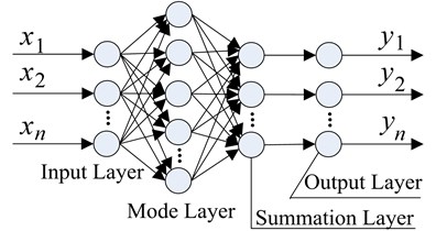
PNN is a feed forward neural network that takes Bayesian risk criteria (namely Bayesian decision theory) as the theoretical basis. This algorithm evolved from the radial basis function network. The basic structure of its hierarchical model is shown in Fig. 2. The PNN consists of 4 layers, which are the input layer, mode layer, summation layer, and output layer.

Fig. 2PNN structure

Given failure modes $θ_{a}$ and $θ_{b}$ as examples, the corresponding failure characteristic sample to be judged is $X = [\begin{array}{l} x_{1} & x_{2} & \dots & x_{n} \end{array}]$ . The following formula was obtained according to the minimum risk Bayes decision rule [22]:

18

\{\begin{array}{l} \begin{array}{l} I f & P_{a} L_{a} f_{a} (X) > P_{b} L_{b} f_{b} (X), & t h e n & X \in θ_{a}, \end{array} \\ \begin{array}{l} I f & P_{a} L_{a} f_{a} (X) < P_{b} L_{b} f_{b} (X), & t h e n & X \in θ_{b} \end{array}, \end{array}

where $P_{a}$ and $P_{b}$ are the prior empirical probability of $X$ when it belongs to $θ_{a}$ and $θ_{b}$ , respectively ( $P_{a} = N_{a} / N$ , $P_{b} = N_{b} / N$ ); $N_{a}$ and $N_{b}$ are the number of training samples of fault modes $θ_{a}$ and $θ_{b}$ ; $N$ is the total number of training samples; $L_{a}$ is the cost factor when the fault characteristic sample $X$ that belongs to $θ_{a}$ is mistakenly divided into mode $θ_{b}$ ; $L_{b}$ is the cost factor when the fault characteristic sample $X$ that belongs to $θ_{b}$ is mistakenly divided into mode $θ_{a}$ ; $f_{a}$ and $f_{b}$ are the probability density functions when $X$ belongs to $θ_{a}$ and $θ_{b}$ , respectively. The conditional probability can be calculated by:

19

f_{a} (X) = \frac{1}{(2 π)^{\frac{P}{2}} σ^{P} N_{a}} \times \sum_{j = 1}^{N_{a}} e x p [- \frac{{(X - X_{a j})}^{T} (X - X_{a j})}{2 σ^{2}}] .

In Eq. (19), $P$ is the vector dimension; $N_{a}$ is the number of training samples for $θ_{a}$ ; $X_{a j}$ is the $j$ th training sample vector of $θ_{a}$ ; $σ$ is the smooth coefficient.

3. Simulation and analysis

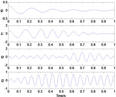
A simulation signal $x_{1} (t)$ is used to test EWT. This simulation signal is composed of two different signals, which are the FM signal $x_{11} (t)$ and the AM signal $x_{12} (t)$ , as shown in Eq. (20):

20

\{\begin{array}{l} x_{11} (t) = c o s (10 π t + 10 π t^{2}) \begin{array}{l} , \end{array} \\ x_{12} (t) = s i n (π t) s i n (30 π t) \begin{array}{l} , \end{array} \\ x_{1} (t) = x_{11} (t) + x_{12} (t) \begin{array}{l} . & \begin{array}{l}  \end{array} \end{array} \end{array}

The time-domain waveform is shown in Fig. 2(a).

The output results of EWT decomposition are obtained by separately filtering of a scaling function and $N$ wavelet functions. Although EMD can automatically estimate mode decomposition layers according to the signal, the empirical wavelet decomposition can set the number of decomposition layers according to different signal requirements. As for simulation signal $x_{1} (t)$ , $N$ is set as 3. Fig. 3(a) and 3(b) show the simulation signal’s time-domain waveform and spectrum and the detected boundary of each filter, respectively.

Fig. 3Simulation signal x1(t)

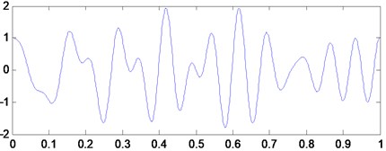
a) Time-domain waveform of simulation signal $x_{1} (t)$

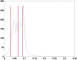
b) Spectrum and support border of simulation signal $x_{1} (t)$

Fig. 4(a) displays the EWT decomposition results of the simulation signal. As seen from the figure, EWT decomposition derives the resolution signal components of the simulation signal and shows the corresponding time-domain signal characteristics. This approach is conducive to further signal processing and analysis.

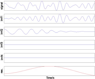
For a comparative analysis with the EMD, Fig. 4(b) shows the EMD results of the simulation signal $x_{1} (t)$ . Fig. 4(b) shows that the simulation signal $x_{1} (t)$ is decomposed into four mode function components and one remainder. According to EMD, the simulation signal $x_{1} (t)$ consists of 4 empirical mode components. Although EMD can automatically estimate the number of mode decomposition layers according to the signal, the number of decomposition layers is significantly higher than that of EWT decomposition; thus, more time is required for consumption calculation, thereby affecting the performance of the algorithm. Among the decomposed excessive modal components, some modal information components have the same composition, and some false modal components are present. These false modal components do not exist in the original signal and will affect the accurate analysis of the signal. In addition, the excessive decomposition layers require more iterations, thereby increasing the amount of computation. Therefore, the amount of EWT calculation is far less than that of EMD for most signals.

Fig. 4EWT mode decomposition results of simulation signal x1(t)

a) EWT mode decomposition of simulation signal $x_{1} (t)$

b) EMD of simulation signal $x_{1} (t)$

In Fig. 4(a), two high-frequency modal components in the middle portion have the same information, but the two modal components with independent energies derived from EWT decomposition can be regarded as two independent resolution-mode components. Fig. 4(b) shows that EMD only decomposes the high-frequency modal component IMF1, thereby leaving the excessive false modal components IMF3, IMF4, and the remainder. Therefore, EWT can extract different modal components from the signal and analyze the different frequency modal components of the signal. Each modal component has more substantial characteristic energy of the original signal. Theoretically, the IMF of each resolution derived from EMD does not guarantee strict orthogonality but can only approximate orthogonality; no complete rigorous theoretical proof can support this. Therefore, modal aliasing phenomena will occur during decomposition. This trend may be due to unreasonable mode decomposition termination conditions and defects in the screening method. However, EWT is a framework based on wavelet theory, which has a solid theoretical foundation. The completeness and orthogonality can be verified and understood by the wavelet transform.

Fig. 5Time-frequency spectrum of the simulation signal x1(t)

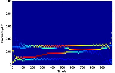
a) EWT-Hilbert spectrum

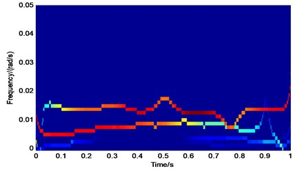
b) EMD-Hilbert spectrum

The Hilbert transform of Fig. 4(a) and 4(b) are performed according to Eq. (13); the corresponding time-frequency energy spectra are obtained and shown in Fig. 5(a) and 5(b), respectively. The Hilbert energy spectrum of the original signal is manifested in a color coded map for time-frequency-amplitude. The magnitude of energy is expressed in its logarithmic form, and deeper colors represent greater energy; otherwise, the energy is smaller. From Fig. 5(a), the simulation signal $x_{1} (t)$ takes angular frequencies of 0.016 and 0.008 rad/s for the main components. The energy spectrum around the angular frequency of 0.016 rad/s is reflected in the cyclical form of sinusoidal oscillation as characterized by the remarkable energy. Fig. 5(b) also has angular frequencies of 0.016 and 0.008 rad/s as the main components. The energy spectrum around the angular frequency of 0.016 rad/s has stable intensity, but the angular frequency has some fluctuations caused by different types of EWT decomposition. Although EMD may generate excessive IMF false components during mode decomposition, the false modal component IMF3 is similar to IMF4; thus, Fig. 5(b) does not reflect more differences.

4. Experiment and analysis of wind power generator vibration signal

4.1. Hardware platform

The comparable motor vibration signals have little differences. The experimental data of Case Western Reserve University are used in the analysis to test the de-noising effect of the EWT-based de-noising method on vibration signals of wind power generators. The database signals are mainly based on the bearing vibration. The experiment platform is set up, including one 2 Hp motor (left), one torque sensor (middle), one power meter (right), and an electronic control device. The tested shaft is a motor shaft. The various fault vibrations of the experiment database are derived by electrical discharge machining technology to simulate single-point failure of the bearing, such as the inner ring, outer ring, and the rolling element of the bearing. Experimental data are collected at different rotation speeds and in different faults.

In the experiment, acceleration sensors are used to collect vibration signals based on the magnetic base, whereas a sensor is installed on the motor shell. The acceleration sensors are mounted on the drive of the motor shell and in front of the fan. In some experiments, the sensor is installed on the motor-supporting chassis. Vibration signals are collected by a 16-channel DAT recorder, and the sampling frequency is 12 000 Hz. For the fault data of the bearing installed on the driving device, the sampling frequency is 48 000 Hz.

4.2. Experimental results and analysis

Data are analyzed according to the experiment on an active bearing 6205-2RS JEM SKF. When the motor load is 3 Hp, the rotational speed is 1730 rpm, and the sampling frequency is 12 kHz. In the absence of fault, the vibration signal time-domain diagram is shown in Fig. 6(a), which shows that the vibration signal contains noise.

For the same motor, the fault diameter is 21 mils and set in the 6 o’clock of bearing’s outer ring, motor load is set as 3 Hp, motor rotation speed is 1730 rpm, and sampling frequency is also 12 kHz. The time-domain diagram of the vibration signal is shown in Fig. 7(a), whereas Fig. 7(b) shows the modal components after EWT decomposition. Fig. 7(a) and 6(a) show that under fault conditions, vibration signals have significant characteristics and have periodicity. Fig. 7(b) and 6(b) are decomposed to generate 4 empirical mode components; these mode components contain high- and low-frequency information of vibration signals.

To analyze and compare the results of EMD and EWT for actual vibration signals, Fig. 7(a) is decomposed by EMD; the empirical mode function is obtained and shown in Fig. 7(c). The figure shows that the vibration signal is decomposed into 10 IMF components and 1 remainder. The first IMF component separates the major vibration signal components and contains noise. This component decomposes into successive IMF components. Although the second IMF component reflects some vibration information, the other IMF components do not have vibration characteristics and cannot be explained. These components can be considered to be in the false mode, which is not conducive to the further decomposition of vibration signals for obtaining characteristic quantities.

Fig. 6Analysis of experimental vibration signal

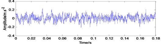
a) Vibration signal waveform in normal time

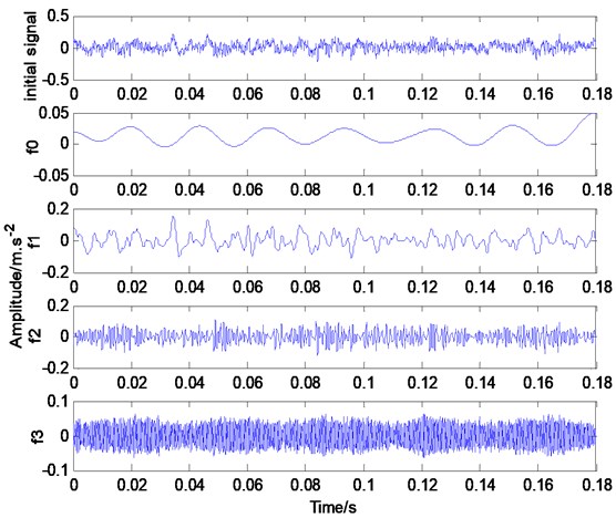
b) Waveform diagram of signal in a) after WET decomposition

The Hilbert transform of Fig. 6(b), 7(b), and 7(c) is performed and the corresponding time-frequency energy spectra are obtained and shown in Fig. 8(a)-8(c), respectively. Fig. 8(a) shows that the vibration signal has three dominant frequency components. Fig. 8(b) takes 0.3 Hz as the predominant component, with a continuous amplitude and significant reflection; however, some energy components are below 0.1 Hz, but they are very weak.

Some significant energy spectra at 0.3 Hz are shown in Fig. 8(c), but these are scattered and discontinuous. Some energy components between 0.05 Hz and 0.3 Hz are very weak and irregular. In addition, some energy components below 0.05 Hz increase in amplitude but with obvious aliasing distortions because excessive virtual IMF components are decomposed and aliasing occurs with the low frequency of the original signal.

The above analysis implies that under fault conditions, the EWT time-frequency energy spectrum of the vibration signal has obvious characteristics, and the EWT time-frequency energy spectrum of the vibration signal can significantly better reflect the characteristics of the original vibration signal than the EMD time-frequency energy spectrum. The mode components derived from EWT decomposition can be combined with the time-frequency energy spectrum to extract the characteristics of the resolution component energy of the vibration signals. This step may facilitate further fault diagnosis and analysis of wind power generator vibration according to the characteristics of vibration signals.

Fig. 7Analysis chart of the experimental vibration signal

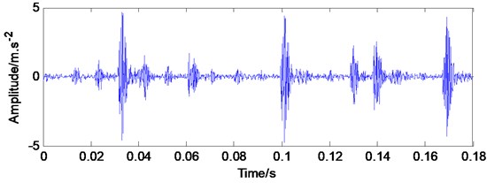
a) Vibration signal waveform when failure diameter is 21 miles

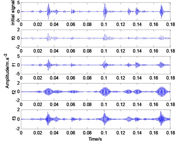
b) Waveform of signal in a) after EWT decomposition

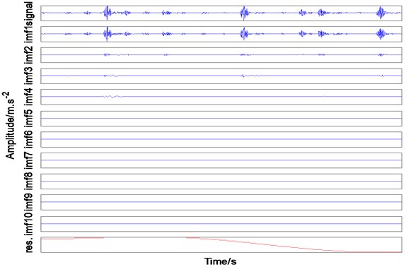
c) Waveform signal in a) after EMD decomposition

The experiment sets three fault types: the inner ring fault, the outer ring fault, and the rolling element fault. These fault vibration signals are collected under the condition where the motor load is 3 Hp, the motor rotation speed is 1730 rpm, and the sampling frequency is 12 kHz. The characteristics mentioned in Section 1.2 are used to extract the characteristics of the EWT component energy under three fault conditions and normal condition; these results are shown in Table 1. The table shows that each type of vibration signal contains four EWT components to form a 4-dimensional vector. By assuming that $X_{1} = [\begin{array}{l} E W T_{1} & E W T_{2} & E W T_{3} & E W T_{4} \end{array}]$ , the input feature sample of the PNN model is used for motor vibration fault analysis. For the PNN classifier output, 1 represents the normal condition, 2 represents the inner ring fault, 3 represents the outer ring fault, and 4 represents the rolling element fault. In the experiment, 33 groups of samples of motors under normal circumstances, the inner ring fault, the outer ring fault, and the rolling element fault are respectively selected; 23 groups of samples are used for training, whereas 10 groups of samples are used for verification.

Fig. 8Time-frequency energy spectrum of vibration signal

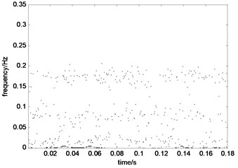
a) EWT time-frequency energy spectrum of normal signal

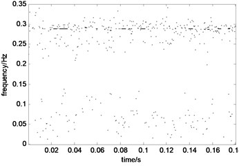
b) EWT time–frequency energy spectrum when fault diameter is 21 miles

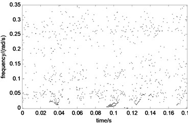
c) EMD time–frequency energy spectrum when fault diameter is 21 miles

Table 1Vector elements of different vibration signals after normalizing EWT energy

Signal	$E W T_{1}$	$E W T_{2}$	$E W T_{3}$	$E W T_{4}$
Normal	0.12242	0.71916	0.56086	0.39148
Inner ring fault	0.056068	0.25514	0.33829	0.90406
Outer ring fault	0.10038	0.84204	0.40216	0.3452
Rolling element fault	0.094096	0.44775	0.66059	0.59522

The expansion speed and smoothing factor of the radial basis function of PNN was adjusted. The spread was 1.1. The four types of characteristics for the 23 sets of training samples are input into the PNN1 model for network training, and a nonlinear corresponding PNN1 network is established. The training classification results are shown in Fig. 9(a); “○” represents the faulty element of the PNN1 network discrimination, whereas “*” represents the actual fault type of power generator vibration. Fig. 9(b) shows the fault identification error and the training classification error.

After training, 10 groups of samples are used as input vectors and substituted into the trained PNN1 for verification and classification. The results are shown in Fig. 9(c), which shows only one fault identification error.

The results indicate that one group difference error still exists even after training the given motor vibration fault samples. The PNN1 can achieve 90 % accuracy rate when classifying samples. However, the vibration fault sample library may be limited, which renders the PNN network training limited. Consequently, 100 % accuracy rate cannot be reached. The next step should be to increase the vibration fault sample library and further improve the superiority of PNN network classification identification.

Similarly, the Eqs. (15)-(17) are used to extract the energy characteristics of each IMF component of the vibration signals for the same data samples. And the first 4 IMF energy components of each signal can be obtained respectively. That is, $X_{2} = [\begin{array}{l} I M F_{1} & I M F_{2} & I M F_{3} & I M F_{4} \end{array}]$ . Taking the same expansion speed and smoothing factor, the four types of characteristics for the 23 sets of the same training samples based on EMD are input into the PNN2 model for network training. After training, 10 groups of same samples based EMD are used as input vectors and substituted into the trained PNN2 for verification and classification. The correct rate of fault identification is shown in Table 2, respectively, based on EWT and EMD. Compared with the results of identification, it can be found that the fault diagnosis method based on EWT is better than the EMD method in the classification of the actual fault data.

Fig. 9PNN-based power generator vibration fault classification

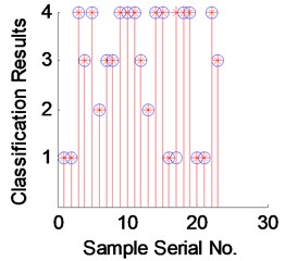
a) Results of classification practice

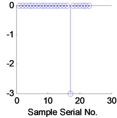
b) Error of classification practice

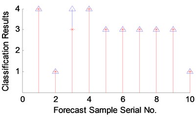
c) Verification of classification results

Table 2The fault identification rate based on EWT and EMD

Method	Normal	Inner ring fault	Outer ring fault	Rolling element fault	Accuracy
EMD	100 %	96.35 %	91.41 %	92.17 %	94.98 %
EWT	100 %	97.62 %	94.86 %	91.93 %	96.10 %

5. Conclusions

EWT is a novel tool for analyzing and processing of nonlinear and nonstationary signals. This paper introduces the advantages of EWT theory, considers the characteristics of the power generator vibration signal, and proposes an EWT-based method to analyze the vibration signal characteristics and to diagnose faults. By conducting the simulation signal and vibration signal experiments, this paper analyzes the HHT mode decomposition and time-frequency energy spectrum under the same signal. For some signals, the number of layers derived from the EWT mode decomposition is less than the number of layers derived from EMD. This value is justified by the complete support wavelet theory and avoids the modal aliasing of EMD. However, the resolution components derived from EWT decomposition have corresponding time-domain signal characteristics, which can facilitate the further analysis of signals. The time-frequency energy spectrum of EWT-based vibration signals can better reflect the characteristics of the original vibration signal than the HHT-based time-frequency energy spectrum.

In addition, the energy normalization of the EWT modal component is defined as the input feature sample of the PNN classifier. Vibration fault diagnosis was conducted according to the PNN classifier. Given the limited training samples, the PNN can achieve 90 % accuracy rate when classifying and judging validation samples. In the classification of the actual fault data, the method based EWT is better than that based on EMD, and it is an effective method for intelligent fault diagnosis. The next steps are to increase the vibration fault sample database. Increasing the PNN samples support its superiority in classification and identification, as well as further improve the diagnostic accuracy in practice. Moreover, other faults, like unbalance and misalignment, will be used to examine the proposed approach in our future research.

References

de Azevedo H. D. M., Araujo A. M., Bouchonneau N. A review of wind turbine bearing condition monitoring: state of the art and challenges. Renewable and Sustainable Energy Reviews, Vol. 56, 2016, p. 368-379.

Publisher
Stone G. C. Condition monitoring and diagnostics of motor and stator windings – a review. IEEE Transactions on Dielectrics and Electrical Insulation, Vol. 20, Issue 6, 2013, p. 2073-2080.

Publisher
Liu W. Y., Tang B. P., Han J. G., et al. The structure healthy condition monitoring and fault diagnosis methods in wind tur-bines: a review. Renewable and Sustainable Energy Reviews, Vol. 44, 2015, p. 466-472.

Publisher
Long Huan, Wang Long, Zhang Zijun, et al. Data-driven wind turbine power generation performance monitoring. IEEE Transactions on Industrial Electronics, Vol. 62, Issue 10, 2015, p. 6627-6635.

Publisher
Garcia Marquez F. P., Mark Tobias A., Pinar Perez J. M., et al. Condition monitoring of wind turbines: techniques and methods. Renewable Energy, Vol. 46, 2012, p. 169-178.

Publisher
Ciang C. C., Lee J. R., Bang H. J. Structural health monitoring for a wind turbine system: a review of damage detection methods. Measurement Science and Technology, Vol. 19, Issue 12, 2008, p. 122001.

Publisher
Maryam A., Hamidreza A. Statistical modeling and denoising Wigner-Ville distribution. Digital Signal Processing, Vol. 23, Issue 2, 2013, p. 506-513.

Publisher
Wu J. D., Huang C. K. An engine fault diagnosis system using intake manifold pressure signal and Wigner-Ville distribution technique. Expert Systems with Applications, Vol. 38, Issue 1, 2011, p. 536-544.

Publisher
Ziaja A., Antoniadou I., Barszcz T., et al. Fault detection in rolling element bearings using wavelet-based variance analysis and novelty detection. Journal of Vibration and Control, Vol. 22, Issue 2, 2016, p. 396-411.

Publisher
Attoui Issam, Omeiri Amar Fault diagnosis of an induction generator in a wind energy conversion system using signal processing techniques. Electric Power Components and Systems, Vol. 43, Issue 20, 2015, p. 2262-2275.

Publisher
Asadi Nahid, Kelk Homayoun Meshgin Modeling, analysis, and detection of internal winding faults in power transformers. IEEE Transactions on Power Delivery, Vol. 30, Issue 6, 2015, p. 2419-2426.

Publisher
Pelegrina G. D., Duarte L. T., Jutten C. Blind source separa-tion and feature extraction in concurrent control charts pattern recognition: Novel analyses and a comparison of different methods. Computers and Industrial Engineering, Vol. 92, 2016, p. 105-114.

Publisher
Au M., Agba B. L., Gagnon F. Fast identification of partial discharge sources using blind source separation and kurtosis. Electronics Letters, Vol. 51, Issue 25, 2015, p. 2132-2133.

Publisher
El Rhabi M., Fenniri H., Keziou A. A robust algorithm for convolutive blind source separation in presence of noise. Signal Processing, Vol. 93, Issue 4, 2013, p. 818-827.

Publisher
Huang N. E., Shen Z., Long S. R., et al. The empirical mode decomposition and the Hilbert spectrum for nonlinear and nonstationary time series analysis. Proceedings of the Royal Society of A: Mathematical, Physical and Engineering Sciences, Vol. 454, 1998, p. 903-995.

Publisher
Laila D. S., Messina A. R., Pal B. C. A refined Hilbert-Huang transform with applications to interarea oscillation moni-toring. IEEE Transactions on Power Systems, Vol. 24, Issue 2, 2009, p. 610-620.

Publisher
Ozgonenel O., Yalcin T., Guney I., et al. A new classification for power quality events in distribution systems. Electric Power Systems Research, Vol. 95, 2013, p. 192-199.

Publisher
Jérôme Gilles Empirical wavelet transform. IEEE Transactions on Signal Processing, Vol. 61, Issue 16, 2013, p. 3999-4010.

Publisher
Chen J. L., Pan J., Li Z. P., et al. Generator bearing fault diagnosis for wind turbine via empirical wavelet transform using measured vibration signals. Renewable Energy, Vol. 89, 2016, p. 80-92.

Publisher
Cao H. R., Fan F., Zhou K., et al. Wheel-bearing fault diagnosis of trains using empirical wavelet transform. Measurement, Vol. 82, 2016, p. 439-449.

Publisher
Liu W., Cao S. Y., Chen Y. K. Seismic time-frequency analysis via empirical wavelet transform. IEEE Geoscience and Remote Sensing Letters, Vol. 13, Issue 1, 2016, p. 28-32.

Publisher
Specht D. F. Probabilistic neural networks. Neural Networks, Vol. 3, Issue 1, 1990, p. 109-118.

Publisher
Mohanty S. R., Ray P. K., Kishor N., et al. Classification of disturbances in hybrid DG system using modular PNN and SVM. International Journal of Electrical Power and Energy Systems, Vol. 44, Issue 1, 2013, p. 764-777.

Publisher
Perera N., Rajapakse A. D. Recognition of fault transients using a probabilistic neural-network classifier. IEEE Transactions on Power Delivery, Vol. 26, Issue 2, 2011, p. 944-953.

Publisher
Asadi Asad Abad Mohammad Reza, Borghei Ali Mohammad, Ahmadi Hojat, Minaei Saeid, Beheshti Babak Fuzzy logic based classification of faults in mechanical differential. Journal of Vibroengineering, Vol. 17, Issue 7, 2015, p. 3635-3649.

Search CrossRef

Cited by

Time-varying damage detection in beam structures using variational mode decomposition and continuous wavelet transform

Jing-Liang Liu | Si-Fan Wang | Yu-Zu Li | An-Hua Yu

(2024)

Fault diagnosis of rolling bearing using symmetrized dot pattern and density-based clustering

Hai Li | Wei Wang | Pu Huang | Qingzhao Li

(2020)

About this article

Received

06 July 2016

Accepted

08 January 2017

Published

15 May 2017

SUBJECTS

Fault diagnosis based on vibration signal analysis

DOI

https://doi.org/10.21595/jve.2017.17374

Keywords

vibration measurement

wavelet transforms

feature extraction

wind power

Acknowledgements

This work is supported by the National Natural Science Foundation of China (51477015), the Visiting Scholarship of State Key Laboratory of Power Transmission Equipment and System Security and New Technology (Chongqing University) (2007DA10512714406), the Putian Science and Technology Project (2016G2021), and the Program for Excellent Youth Talents in Fujian Province University (2015054).

This is an open access article distributed under the Creative Commons Attribution License, which permits unrestricted use, distribution, and reproduction in any medium, provided the original work is properly cited.

Previous article in issue Previous Next article in issue Next

Research article

2023 08 01

Rolling bearing fault diagnosis method based on ELMD hybrid feature extraction and wavelet neural network

Hengxin Yue, Xihui Chen, Xinhui Shi, Wei Lou

Research article

2021 09 21

A study on the feature separation and extraction of compound faults of bearings based on casing vibration signals

Qizhi Fang, Baodong Qiao, Mingyue Yu

Research article

2019 09 30

Bearing fault diagnosis based on feature extraction of empirical wavelet transform (EWT) and fuzzy logic system (FLS) under variable operating conditions

Fawzi Gougam, Chemseddine Rahmoune, Djamel Benazzouz, Boualem Merainani

Research article

2019 03 15

Bearing fault analysis using kurtosis and wavelet based multi-scale PCA

Ankush C. Jahagirdar, Satish Mohanty, Karunesh Kumar Gupta

X. Chen, Y. Yang, and N. Yang, “Feature extraction and fault diagnosis of wind power generator vibration signals based on empirical wavelet transform,” Journal of Vibroengineering, Vol. 19, No. 3, pp. 1745–1758, May 2017, https://doi.org/10.21595/jve.2017.17374

Copy Extrica

Copied to clipboard!

TY  - JOUR
DO  - 10.21595/jve.2017.17374
UR  - https://doi.org/10.21595/jve.2017.17374
TI  - Feature extraction and fault diagnosis of wind power generator vibration signals based on empirical wavelet transform
T2  - Journal of Vibroengineering
AU  - Chen, Xuejun
AU  - Yang, Yongming
AU  - Yang, Ning
PY  - 2017
DA  - 2017/05/15
PB  - JVE International Ltd.
SP  - 1745-1758
IS  - 3
VL  - 19
SN  - 1392-8716
ER  - 

Copy Ris

Copied to clipboard!

@article{Chen_2017,
	doi = {10.21595/jve.2017.17374},
	url = {https://doi.org/10.21595/jve.2017.17374},
	year = 2017,
	month = {may},
	publisher = {{JVE} International Ltd.},
	volume = {19},
	number = {3},
	pages = {1745--1758},
	author = {Xuejun Chen and Yongming Yang and Ning Yang},
	title = {Feature extraction and fault diagnosis of wind power generator vibration signals based on empirical wavelet transform},
	journal = {Journal of Vibroengineering}
}

Copy Bibtex

Copied to clipboard!

[1]X. Chen, Y. Yang, and N. Yang, “Feature extraction and fault diagnosis of wind power generator vibration signals based on empirical wavelet transform,” Journal of Vibroengineering, vol. 19, no. 3, pp. 1745–1758, May 2017, doi: 10.21595/jve.2017.17374.

Copy IEEE

Copied to clipboard!

Chen, Xuejun, Yongming Yang, and Ning Yang. “Feature Extraction and Fault Diagnosis of Wind Power Generator Vibration Signals Based on Empirical Wavelet Transform.” Journal of Vibroengineering 19, no. 3 (May 15, 2017): 1745–58. https://doi.org/10.21595/jve.2017.17374.

Copy Chicago

Copied to clipboard!

Feature extraction and fault diagnosis of wind power generator vibration signals based on empirical wavelet transform

Abstract

1. Introduction

2. EWT-based on vibration signal analysis

2.1. EWT method

2.2. Extraction and fault diagnosis of vibration signal characteristics

3. Simulation and analysis

4. Experiment and analysis of wind power generator vibration signal

4.1. Hardware platform

4.2. Experimental results and analysis

5. Conclusions

References

Cited by

About this article

Related Articles