3D meshless FEM-BEM model for prediction of sound fields in cabins due to external sound disturbances

Liu, Yanshan; Zeng, Xiangyang; Wang, Haitao

doi:10.21595/jve.2017.17176

Journal of Vibroengineering

Browse Journal

Submit article

Published: 15 November 2017

Check for updates

3D meshless FEM-BEM model for prediction of sound fields in cabins due to external sound disturbances

Yanshan Liu¹

Xiangyang Zeng²

Haitao Wang³

^{1, 2, 3}School of Marine Science and Technology, Northwestern Polytechnical University, Xi’an, 710072, China

Corresponding Author:

Xiangyang Zeng

Cite the article Download PDF

Downloads 1455

Abstract

The Finite Element Method (FEM) and Boundary Element Method (BEM) are widely applied to predict the sound pressure level (SPL) in enclosed spaces for low frequency problems. However, a single method usually cannot fulfill the task for predicting the internal SPL in enclosures including objects in the interior due to external disturbances. Moreover, these methods have some disadvantages such as complex pre-processing, time-consuming and inevitable pollution effects. Based on these drawbacks, this paper attempts to combine the Meshless Method (MM), acoustical FEM and BEM into a hybrid method which can be applied to predict the SPL in an enclosed environment with external sound sources. Firstly, the hybrid theory for the acoustic problem and its implementation are illustrated. Next, numerical simulations and experiments are conducted to validate the peak value, SPL and computing efficiency using this method. Comparative results obtained from the proposed method, FEM and BEM using SYSNOISE are shown to be in agreement, and the proposed method is more efficient. Experimental results show that the average relative error of SPL in each location is less than 5.26 %. It is corroborated that the proposed method is applicable to the prediction of the internal SPL with the case of exterior sound sources existed.

1. Introduction

A precise prediction of the sound pressure level (SPL) in enclosed spaces can provide theoretical bases to lower the SPL which is a significant index in the quality evaluation of the cabins. The acoustical simulation serves as a high-efficiency measure to make it clear about the acoustic behavior of the complicated structures such as cabins of vehicles or airplanes. More and more efficient methods are developed for acoustic engineers to get useful hints before optimizing the prototyping of the production in aviation and other engineering industry. Therefore, more economical and practical numerical methods are required provided the SPL are computed exactly and efficiently for complicated structures or acoustic fields.

The finite element method (FEM) and boundary element method (BEM) are low-frequency numerical methods which are widely used for the prediction of the internal SPL in enclosed space [1-4]. But there are some restrictions when they are applied in such two circumstances. One is that desks, seats or lump-shaped vibrating objects exist in the internal space. This can be solved by multidomain FEM and BEM. However, the data transmission of the different domains is a troublesome process especially for several contacted surfaces with sharp shapes. Another one is the internal sound field generated by some external sources. Although that solution can be obtained by BEM and FEM, but some difficulties are unavoidable for FEM or BEM. FEM can provide a desired distribution of SPL for the exterior problem at the cost of dealing with many more freedoms than BEM, and BEM is applied in internal sound pressure computing with low-frequency breakdowns and artificial damping due to discretization errors [5]. Fortunately, the integrated FEM-BEM method is proposed to predict the structural acoustic radiation [6, 7] in which the dynamic response of the structure is determined by FEM and the acoustic field is obtained by BEM. Based on FEM-BEM method, the boundary condition for the external acoustic simulation can be obtained and the internal SPL is determined using FEM after mapping the data between the nodes of the finite domain and those of the boundary domain. However, there are some ineluctable disadvantages for the FEM-BEM similar to that for FEM and BEM methods. Several deficiencies are inherently inevitable in the numerical simulation with the FEM and BEM such as the upper frequency due to the spatial discretization of the problem domain, the preprocessing and post-processing in the wave-based methods which require a lot of time especially for complicated shapes.

The meshless method is a potential solution to mitigate those restrictions. The meshless method proposed four decades ago uses only a certain cluster of nodes to solve the astrophysical problems [8] for the flexibility and simplicity. In the 2000s, it was introduced into acoustics for vibro-acoustic [9], acoustical radiation and scattering problem [10, 11]. In 2012, there were some new hybrid methods synthesizing of FE and meshless methods, the FE-LSPIM was applied to solve the interior SPL in 2D plane [12]. Recently, the meshless method was proposed to solve unbounded acoustic problems [13] and three-dimension exterior acoustic problems with irregular domains [14]. Meanwhile, the meshless method in mechanics [15] was introduced into the numerical acoustics for cabin sound field modeling [16] for author’s research. However, current models cannot simulate the prediction of the internal SPL if the sound source was located in the exterior of the cabin in which some lump-shaped objects existed. As a consequence, this paper settles the previous described FEM-BEM problems with a modified FEM-BEM method. The mathematical model used in meshless methods is derived by the Galerkin method to overcome the aforementioned time-consuming and tedious preprocessing in the simulation. The shape of the node distribution can be applied to structures or acoustic cavities with arbitrary geometry and the mesh process is eliminated. The most expectation is the accuracy improvement and fitness for the local predictions. Thus, the modified MFBM (Meshless method, FEM and BEM) is proposed.

In this paper, the hybrid theory of the method which combines the meshless method with FEM and BEM is specified in Section 2. Section 3 simulates the sound field in a rectangular and cylinder cavity which is also simulated in SYSNOISE with the FEM and BEM as contrasts to verify the feasibility of the algorithm. Section 4 validates the veracity of the proposed numerical method through the measurements in a cabin structure. It should be noted that the wave equation, boundary integral equation and boundary condition involved in the following sections are analyzed in the frequency domain.

2. Hybrid theory for acoustic problem

Solving partial differential equations of the acoustic wave equations is essentially a numerical SPL prediction for practical acoustic engineered applications. The hybrid method which consists of MMFEM (meshless combined with FEM) and MMBEM (meshless combined with BEM) is proposed in this paper. The meaning of the combination is that the computation is implemented in two phases. The main phase is the process of MMFEM, and the MMBEM is implemented to determine the boundary velocity. The shape function in the MMFEM and MMBEM is constructed by the meshless method, along with the coordinates of those meshless nodes and integral points.

The meshless method can also be named as MM (meshfree method) or EFM (element free method) [17]. The shape function involved in the meshless method is constructed as follows. Firstly, the coordinates of nodes of the geometric model are designed to approximate the SPL in the problem domain. Secondly the nodal weight function or kernel function is selected to relate the desired SPL of the node to its corresponding nodes in the nodal neighborhood. The neighborhood can also be named as a support domain specified by a weight function. The SPL in the influence domain can be approximated based on the weight function and shape function. Finally, the shape function can be determined through the approximation of interpolation with different nodal neighborhood.

The numerical calculations of the two combined models are carried out in three steps. Firstly, the weighted residual method or the variation method is utilized to transform the acoustic wave equation into an equivalent integral equation. Then the problem domain is discretized with a certain number of nodes and appropriate distribution of integral points. Next, the shape function is calculated based on the coordinates of the nodes and integral points mentioned in the above paragraphs. Finally, the predefined boundary condition is assigned at the nodes of the boundary domain, and the SP approximated for different nodes can be obtained by solving the linear equations which consist of the aforementioned matrices.

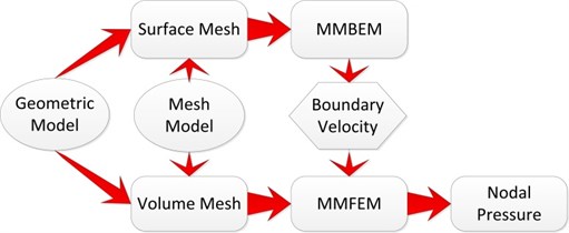
As highlighted in the above argument, obtaining the SPL in the cabin is the main purpose when the sound source is located out of the cabin. As such this paper introduces the meshless method into the conventional FEM-BEM hybrid theory. Fig. 1 illustrates the main principle of the hybrid method. Firstly, the meshless method and BEM are combined to give an insight into the boundary velocity of the cabin or other structures due to external sources. The involved theory of this phase is listed in Section 2.1 and 2.2. Secondly, based on the obtained data on the boundary surfaces in the first step, the meshless method and FEM are combined to obtain the variables of the sound field of the interior domain of the cabin and the specific details are listed in Section 2.1 and 2.3. Based on the first combination, the normal velocity on the outer boundary of the cabin can be determined for the exterior domain, then the interior SPL can be computed with the second combination. Finally, the SPL in any internal location of the cabin can be determined by the interpolation of the shape function. To illustrate the hybrid method, the basic theory of the meshless method is first depicted, then the MM-FEM and MM-BEM are explained respectively in the following sections.

Fig. 1Schematic diagram of meshless FEM-BEM

2.1. Compactly supported trial function for meshless method

There are currently several different forms of meshless methods. The main differences are equivalent integral forms and discrete ways of the partial differential equations which are based on the wave formulation of the practical application [17]. The weighted residual method based on the equivalent integral form of the differential equation can provide a highly efficient solution to the partial equation. The similar system equation can be derived in the meshless method using the weighted residual method or the variation method [18]. The most common weight functions in the meshless method include collocation methods, least square method, and Galerkin method. The Galerkin weighted residual method is applied to construct the system equation [17] in the subsequent calculation.

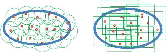
The discrete form of differential equations can be determined by the shape function that is a trial function defined in the support domain of the node. The value of the shape function of the nodes in the exterior of support domain is zero. As to 2D problems, the geometric shapes of the domain generally are circular or rectangle as depicted in Fig. 2. The blue lines and green lines denote the boundary domain and support domain respectively. After the coordinates of nodes are determined, each node has a circular, rectangular or other support domain which is significant to construct the shape function. The SPL at the nodal location can be determined by the neighboring node and corresponding weight functions (It should be noted that this weight function is different from that in the weighted residual method).

The weight function generated by the node $x_{I}$ is a compactly supported function defined within the local domain of the weight function $w (x - x_{I}) \neq 0$ . The weight function is a function of the spatial distance, that is $w (x - x_{I}) = w (d)$ , and $d$ is the distance vector from all the influential points in the local supported domain to the node $I$ . Commonly used weight functions include the exponential weight function, cubic spline weight function, quartic spline weight function and B-spline weight function and so on. The cubic spline weight function has been applied in the proposed method.

Fig. 2Nodal compactly supported domain

In the problem domain, the sound pressure in an arbitrary location can be represented by the following equation:

1

p (x) \approx p^{h} (x) = \sum_{I = 1}^{n} N_{I} (x) \cdot p_{I} = N^{T} \cdot p .

In Eq. (1), $n$ is the number of discrete nodes. $P_{I}$ is the value of sound pressure at the node $x_{I}$ . $N$ and $p$ are given as follows:

2

N = [N_{1} (x), N_{2} (x), \dots, N_{N} (x)],

3

p = {[p_{1}, p_{2}, \dots p_{N}]}^{T} .

All the contributions of nodal sound pressure from other nodes can be computed by the meshless method to obtain the unknown pressure in any location, while in the FEM, only the contributions from the nodes included in the mesh element corresponding to the desired location are computed. In this context, the computational data using the meshless method is more than those using the FEM, which will be demonstrated in the following section. However, if the stiffness matrix and mass matrix arecomputedusing the meshless method, the assembling process is needless and complex mesh process will be simplified.

Based on the shape function constructed using the MLSM (moving least square method), FEM and BEM can be modified and combined with the meshless method. The details of MLSM can be found in [16]. The implementation of the hybrid mathematical model is listed as follows.

2.2. Mathematical formulations for modified meshless FEM model

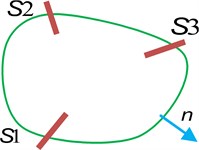
Let’s suppose an enclosed space shown in Fig. 3 with a volume of $V$ , a total area of $S$ . $S 1$ , $S 2$ , $S 3$ are indexed as the rigid boundary surface, absorption boundary surface and velocity boundary surface respectively. $n$ is the out forward normal direction of the structure.

The acoustic boundary condition is defined as follows:

The normal gradient of pressure on the $S 1$ surface:

4

\frac{\partial p}{\partial n} = 0 .

The normal gradient of pressure on the $S 2$ surface:

5

\frac{\partial p}{\partial n} = - j ρ ω \frac{p}{Z_{S}} .

The normal gradient of pressure on the $S 3$ surface:

6

\frac{\partial p}{\partial n} = - j ρ ω v_{n} .

Fig. 3Schematic of enclosed space

The computation of the SPL in the enclosure mathematically solves a second-order partial differential equation of the acoustic wave equation defined in the internal domain of the structure with the inhomogeneous boundary condition. Introducing the Galerkin method into the hybrid method, the system equation can be discretized and integrated as follows [16]:

7

(K + j ρ ω C - k^{2} M) p = F,

where $K$ , $C$ , $M$ , $F$ are stiffness matrix, damping matrix, mass matrix and load vector respectively. The shape function in this paper is calculated using the MLS method [16] after discretizing the structure model and obtaining the nodal coordinates. Note that the algebraic expression is different from the conventional methods because of the MLS shape function. After substituting the MLS shape function into the system equation, the desired discrete matrix is computed as follows:

8

K = \sum_{i = 1}^{n} ω_{i} \nabla N_{i} \nabla N_{i}^{T},

9

M = \sum_{i = 1}^{n} ω_{i} N_{i} \cdot N_{i}^{T},

10

C = \sum_{i = 1}^{l} ω_{i} N_{i} \cdot N_{i}^{T} / Z_{s},

11

F = - j ρ ω v_{n} \sum_{i = 1}^{m} ω_{i} N_{i},

where $n$ , $l$ is the number of the integral point in the volume and the integral point at the impedance boundary, and $m$ is known as the number of the integral point at the velocity boundary. $ω_{i}$ is the weighted coefficient of the Gauss point of the surface or volume to the node in the integral process, and $N$ is the aforementioned shape function whose element is the contribution from an integral point in the integral surface or the volume to a node in the volume.

Assuming that the positional distribution of the node is determined, the MLS shape function of each node can be obtained from every Gauss point. The aforementioned boundary condition can be substituted into Eq. (10) to compute the damping matrix, and Eq. (6) is substituted into Eq. (11) to obtain the load vector using the meshless BEM explained in the next section. Then the distribution of the sound field in any location can be computed by solving the linear Eq. (7). In practical engineering, the space occupied by seats or other absorption objects is always referred as a cavity encapsulated in the external acoustic domain, and the distinction is that the material is foam or other isotropic material.

2.3. Mathematical formulations for modified meshless BEM model

For the exterior domain, the sound pressures in any position are satisfied with the Kirchhoff-Helmholtz equation:

12

c (P) p_{ω} (P) = \int_{\partial Ω} p_{ω} (Q) \frac{\partial G (P, Q)}{\partial n_{Q}} d \partial Ω - \int_{\partial Ω} G (P, Q) \frac{\partial p_{ω} (Q)}{\partial n_{Q}} d \partial Ω + j ρ ω q_{ω} (r_{0}) G (P, r_{0}),

where $P$ represents the point in the domain or on the boundary, $Q$ is the integral point. The matrix $C$ formed by the coefficient $c$ of point $P$ is given as follows:

13

C = [\begin{matrix} c (P_{1}) & 0 & \dots & 0 \\ 0 & c (P_{2}) & \dots & 0 \\ ⋮ & ⋮ & ⋱ & ⋮ \\ 0 & 0 & \dots & c (P_{n}) \end{matrix}],

where $α$ is the solid angle at $P$ .

The boundary of the solution domain can be divided into a certain number of nodes. The system equation can be written as follows [19]:

14

C p = G p - H p + F,

where $G$ and $H$ are the influence matrix formed by the contribution of each node from each integral point in the other location, and $F$ represents the exciting matrix obtained by the monopole or other sound source, and $p$ is a sound pressure column vector, and $P_{I}$ is the contribution at node $I$ ( $I =$ 1, 2, 3,…, $n$ ) from all the integral points or Gaussian quadrature points. The mentioned matrix can be written as follows:

15

G = [\begin{array}{l} G_{11} & G_{12} & \dots & G_{1 m} \\ G_{21} & G_{22} & \dots & G_{2 m} \\ ⋮ & ⋮ & ⋱ & ⋮ \\ G_{n 1} & G_{n 2} & \dots & G_{n m} \end{array}],

16

G_{i j} = ω_{i j} \frac{1}{4 π r (i, j)} e x p (- j k r (i, j)) \frac{\partial r (i, j)}{\partial n},

17

H = [\begin{array}{l} H_{11} & H_{12} & \dots & H_{1 m} \\ H_{21} & H_{22} & \dots & H_{2 m} \\ ⋮ & ⋮ & ⋱ & ⋮ \\ H_{n 1} & H_{n 2} & \dots & H_{n m} \end{array}],

18

H_{i j} = ω_{i j} \frac{1}{4 π r (i, j)} e x p (- j k r (i, j)),

19

F (ω) = j ρ ω q (r_{0}) G (P, r_{0}),

20

p = \sum_{j = 1}^{m} N (j, I) \cdot p_{I},

where Eq. (16) and Eq. (18) are the representation of influence matrices, and $i$ , $j$ is the serial number of the node and the integral point respectively. The influence matrix is obtained through the ergodic process with respect to each node. The system equation in the meshless BEM can be determined by substituting the corresponding matrix into Eq. (12). Then all the variables on the boundary can be obtained by solving the system of linear equations using the Gauss elimination method or other solution methods. The prediction of SPL in any positions in the domain can be implemented using the boundary variables relationship through Eq. (12). Finally, the normal velocity of the node on the boundary can be determined.

2.4. Data relation in hybrid process

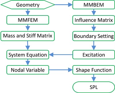
The meshless method is combined with the FEM and BEM in the proposed hybrid method. As for the MMBEM, the geometry model is discretely represented using a cluster of nodes firstly which means that the coordinate of the nodes and integral points is determined. Then the different influence matrix can be obtained after traversing all the node and integral points. Finally, the normal boundary velocity is computed through Eq. (11) and its relationship with sound pressure on the boundary. Likewise, in the MMFEM phase, the nodal position in the meshless method is generated firstly, then the corresponding matrix is integrated according to the integral discretization. In the end, the distribution of the SPL for each node is determined through the equation Eq. (7) after inserting the boundary condition into the equation. Fig. 4 depicts the data flowchart in the hybrid process.

Fig. 4Data flowchart for the hybrid method

3. Numerical simulation

To validate the proposed method, three examples are listed to illustrate the comparison of the results by the proposed method and that obtained from SYSNOISE which is a mature commercial software based on FEM and BEM. Case 1 is to illustrate the simulation of SPL in a regular cylinder with an external sound source. Case 2 is a simulation for a rectangular enclosure with a small-scale box in the internal space and with an external sound source. Case 3 is the qualitative evaluation about the computing time and resource used in a rectangular enclosure. The details can be found as follows.

3.1. Circular cylinder with two closed end caps

As in the aforementioned argument, the diagram of the cylindrical shell structure and location of sources and receivers are depicted in Fig. 5. The radius and axial length of the cylinder are 1m and 3 m. The origin of coordinates is located at the center of the left end-cap. The location of the sound source is (3, 0, 1.5), and the volume velocity is set to 1. The receiver positions of $p 1$ , $p 2$ , $p 3$ are (0, 0, 0.9), (0, 0, 1.5), and (0, 0, 2.1) respectively. The impedance of each surface of the cabin is 200 $ρ_{0} c_{0}$ , in which $ρ_{0}$ is 1.225 kg/m³, and the air density at a normal room temperature under the standard atmospheric pressure, and $c_{0}$ is the sound propagation velocity at a room temperature respectively.

Fig. 5Schematic of cylindrical shell structure

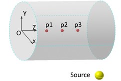
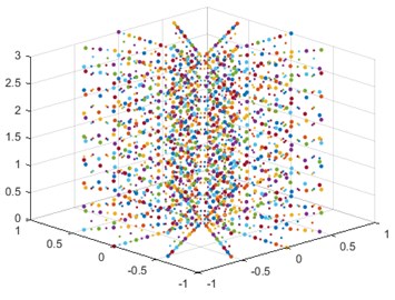
Fig. 6 illustrates the nodal distribution of the cylinder. The radius of the support domain is 1.5 m. The same simulation is executed in the SYSNOISE with the FEM and BEM simultaneously with the frequency range of 50-250 Hz.

Fig. 6Nodal distribution of meshless model

The frequency response at different field points in the interior domain is computed in this example. At field points $p 1$ , $p 2$ , $p 3$ , the peak frequencies are about 114 Hz and 208 Hz, and the total SPL at the frequency range for each point are 84.8 dB, 85.0 dB, and 84.8 dB respectively. To validate the accuracy of the proposed method, the data computed by the proposed method are compared with those simulated by FEM and BEM using SYSNOISE.

Fig. 7frequency response of magnitude at p2 (‘MFBM’ represents the result obtained using meshless FEM-BEM method, and ‘FEM’ and ‘BEM’ represents the result from SYSNOISE using FEM and BEM)

frequency response of magnitude at p2 (‘MFBM’ represents the result obtained using meshless FEM-BEM method, and ‘FEM’ and ‘BEM’ represents the result from SYSNOISE using FEM and BEM)

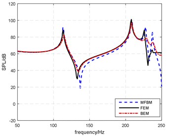
The frequency response of the field point $p 2$ in two methods is illustrated in Fig. 7. The results indicate that the peak value of the sound pressure obtained by the three methods gets close to each other. With regard to the total SPL, the result of the proposed method is 84.8 dB, and the result of FEM and BEM is 88.5 dB and 86.3 dB the errors are 3.7 dB and 1.5 dB with relative errors of 4.4 % and 1.8 %.

It can be attributed to two reasons for that the results get deteriorated as the frequency increase. One is that the higher the computing frequency the more nodes it requires, another one is the nonuniform distribution of nodes for each model and the appropriate value for the support radius in the proposed method. The value for the support radius should always be designated as the 2.8-5.0 times of the average distance of the nodes near the calculation point [16], and in this paper, it is set to 4.1.

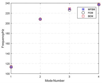
In order to compare the natural frequencies obtained by the proposed method with those obtained using FEM and BEM in SYSNOISE, the natural frequencies are determined by picking the peaks in the curve of Fig. 7. A comparison of natural frequencies is shown in Fig. 8. From the results, the locations of the peak frequency by the three methods are extremely consistent with a little difference for the third mode.

Fig. 8Comparison of natural frequencies calculated by MFBM, FEM and BEM analysis

3.2. Rectangular cavity included small-scale object

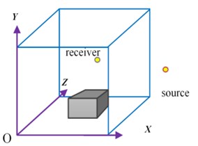
This second numerical example is carried out to validate the prediction case in cabins where other objects exist. This case simulates the sound field in a rectangular cavity, which has dimensions 1 m×1.1 m×1.2 m, and includes a small-scale box with a dimension of 0.5 m×0.55 m×0.24 m. All the absorption coefficients of the boundaries are set to be zero except for the upper wall ( $y 0 =$ 1.1 m), which is 200 $ρ_{0} c_{0}$ . The sound source is a monopole with unit volume velocity as above. (3, 0, 0) and (0.8, 0.6, 0.9) are the locations of the sound source and the receiver respectively. The coordinate of the center of the bottom part of the box is (0.5, 0, 0.6). The density and sound velocity for the box are set to be 22 kg/m³ and 70 m/s. Fig. 9 is the schematic drawing of the rectangular space.

Fig. 9Schematic drawing of rectangular space

The same numerical simulation is carried out with the proposed method, FEM and BEM in SYSNOISE as above. For the model in SYSNOISE, the numbers of the element, node and integral point are125, 216 and 1000, while in the model of the proposed method, the numbers of the node and integral point are 216 and 1000. Fig. 10 illustrates the corresponding results for three methods with the range of 0-300 Hz for the analyzing frequency.

Fig. 10 shows the SPL obtained by MFBM, FEM and BEM. It can be indicated that the peak value obtained by three methods gets close to each other. With regard to the total SPL, the result using proposed method is 88.3 dB, and the result using FEM and BEM is 89.6 dB and 86.2 dB respectively. The relative errors are 1.3 dB and 2.1 dB with absolute percent errors of 1.5 % and 2.3 %. The curve in Fig. 10 shows an excellent agreement can be obtained by three methods.

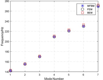
To compare the natural frequencies, the peaks in the curve of Fig. 10 are picked out. A comparison of natural frequency for each method is shown in Fig. 11. As shown in Fig. 11, the frequencies of the peaks for three methods are nearly identical. The frequencies also correspond to the first few acoustic modal coordinates for the rectangular cavity. It is indicated that the sound pressure and peak frequency value can be agreed for these three methods.

Fig. 10Comparison of transfer functions using different methods

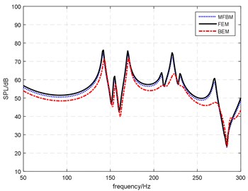
Fig. 11Comparison of natural frequencies calculated by MFBM, FEM and BEM analysis

3.3. Evaluations of efficiency of the method in rectangular cavity

Another case is carried out to evaluate the computing time and resources of the simulation with the proposed method. The sound field in a rectangular cavity with the dimensions of 1 m×1.1 m×1.2 m is simulated. All the acoustic impedance of walls is 25 $ρ_{0} c_{0}$ . The sound source is a monopole with unit volume velocity as above. The coordinates of the sound source and the receiver are kept consistent as above. The rectangular space parameter is also the same as above.

For the sake of evaluating the computational efficiency of the proposed method, the numerical simulation of a rectangular room is carried out with the proposed method and BEM in SYNOISE, as above, in a common computer. The configuration of the computer is Intel Pentium CPU G630 with a RAM of 10 GB. The code for the proposed method is operated in MATLAB R2015a. The number of the nodes of the model in MFBM and SYSNOISE are kept consistentand is designated as 5×5×5 = 125, 6×6×6 = 216, 7×7×7 = 343, 8×8×8 = 512, 9×9×9 = 729, and 10×10×10 = 1000. The range of the analyzing frequency remains 0-300 Hz. The elapsed time is integrated in Table 1.

As shown in Table 1, the elapsed time of each method increases with the number of nodes. The elapsed time of the proposed method is less than that of SYSNOISE. In the last row of the table, MFBM takes a little bit more time than the SYSNOISE.

Table 1Comparison of computing time between proposed methods and SYSNOISE

Number of nodes	MFBM	SYSNOISE
Number of nodes	Time (s)	Time (s)
64	1.6	16.4
125	3.8	35.2
216	9.4	48.7
343	23.1	73.5
512	55.7	113.7
729	120.3	168.6
1000	253.6	238.4

3.4. Discussion of results

With respect to numerical acoustic simulations, the most concerned mainly includes the peak value, total SPL and natural frequencies. In Section 3.1, 3.2 and 3.3, the simulation in different conditions is demonstrated to illustrate the peak value, SPL and natural frequencies of the proposed method in different aspects. The prediction of the SPL in a regular cylinder with an external sound source is illustrated in the first case. The second case is a simulation for a rectangular enclosure with a small-scale box in the internal space and with an external sound source. Qualitative evaluations about the computing time in a rectangular enclosure are illustrated in case 3.3.

The cases in Section 3.1 and 3.2 indicate that the similar peak value and SPL in cubic or cylindrical enclosures can be obtained using the proposed method and the conventional methods (FEM and BEM). However, the cylinder bending surface requires a lot of nodes to model the envelop for the curved surfaces. Therefore, the rectangular cavity can be discretely represented more readily than the cylindrical cavity using a cluster of nodes. Accordingly, the comparison obtains better results for the rectangular cavity. As for the natural frequencies in the results in Section 3.1 with Section 3.2, it is shown that similar results can be obtained for the proposed method and the conventional ones. Based on the evaluation in Section 3.3, it can be concluded that the proposed method has much more potential than the conventional method in the computational efficiency.

It can be concluded that the main advantages of the proposed method with respect to the conventional ones are the convenient pretreatment of the mesh and the satisfying computational efficiency. As a consequence, for 3D interior acoustic computing with an external disturbance, the proposed method can be implemented as a potential one to simplify the pretreatment.

4. Measurement and validation

4.1. Experiments in a circular cylinder with two closed end caps

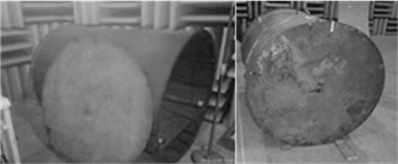
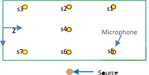
In order to validate the applicability of the proposed model, the sound pressure in a cylindrical cabin structure shown in Fig. 12 is simulated using the proposed method and measured in a semi-anechoic chamber. The sound pressure levels in seven different positions $s 1$ - $s 7$ are recorded in the cabin with the radius of 0.6 m and length of 2.4 m respectively. The structure of the cabin is placed on the floor supported by some wide boards.

The measurement system is configured as Fig. 13 with a Dell-PC, B&K Pulse 3560B and B&K Audio Power Amplifier 2716-C. The source signal is the Gaussian white noise with frequency from 16 Hz to 12.8 kHz played by the omnidirectional spherical sound source B&K 4292, with a distance of 3 m to the boundary of the cabin and a height of 1 m to the floor. Seven BSWA’s MA211 microphones are fixed following as the distribution shown in Fig. 14 with a distance of 10 cm to the upper surface of the model.

Fig. 12Cabin model

4.2. Results and analysis

The measured sound pressure is compared with the simulation by the proposed method. That structure and the model in the simulation are approximately identical and the reflection of the floor is ignored in the simulation. The comparisons of the SPL with different methods, and the error of the sound pressure at field point $s 2$ , are shown in Fig. 15 and Fig. 16.

Fig. 13Schematic of experimental measurements

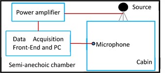
Fig. 14Positional distribution of microphones and source

As shown in Fig. 15 and Fig. 16, at the frequency of 0-200 Hz, the deviation between the numerical results and measurement stays within 5 dB. While at the frequency of 200-500 Hz, the deviation gets larger, with the largest value occurring at 250 Hz. That is caused by two factors. One is that the low order interpolation cannot approximate the sound field in high accuracy in the frequency above 200 Hz, and another one is that the number of required nodes increase with the increase of the required frequency. However, the overall trend suggests that the results of the numerical simulation and measurement at field point $s 2$ are basically consistent.

To determine the total SPL for each field point, the data obtained from numerical and measurement is processed using the logarithmic mean method in the frequency range of 63 Hz-500 Hz. The comparison of the SPL between numerical calculation and measurements is listed in Table 2.

As shown in Table 2, the relative error of SPL for each position of the sensor is below 7.5 %. However, the values in $s 1$ , $s 2$ , $s 3$ , and $s 4$ are slightly more than those in $s 5$ , $s 6$ , and $s 7$ . The dominating influences are the sound reflection from the floor of the semi-anechoic chamber and the sound source in farther distance from $s 1$ , $s 2$ , $s 3$ and $s 4$ . And the cabin contains a lot of stiff ended-plates, and the ribbing structure cannot be intactly modeled in the simulations. Other causes include the difference of the locations in the simulation and measurement, the channel noise induced by the experimental equipment and other background noises, etc.

On the basis of the SPL value at each point, the average relative error for the seven receivers is 5.26 %. These comparisons indicate that simulations by the proposed method are very close to the measurements, and the proposed method can be applied to the prediction of the sound field in the cabin when the sound source is located outside.

Fig. 15SPL comparison at s2

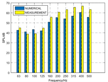
Fig. 16SPL error at s2

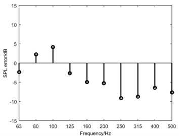
Table 2Comparison between numerical calculation and measurement

Receiver	Total SPL / dB
Receiver	Simulation	Measurement	Relative error
$s 1$	74.0	69.9	5.87 %
$s 2$	78.3	73.4	6.68 %
$s 3$	77.4	72.8	6.32 %
$s 4$	79.7	74.3	7.27 %
$s 5$	71.3	73.7	3.26 %
$s 6$	74.2	72.4	2.49 %
$s 7$	77.6	73.0	4.93 %

4.3. Limitations

It is noted that some conditions should be satisfied to apply the proposed method. Firstly, the proposed method is only applicable for meso-scale and small-scale enclosed structures. The large-scale spaces require geometric acoustical simulations or statistical energy analysis methods. The second item is the upper limiting frequency due to the spatial discretization of the problem domain. The maximum nodal distance shall be at least larger than one sixth of the minimum wavelength to ensure the accuracy of the calculation. The main cause is that the MLS shape function cannot simulate the fluctuations for the high wave number due to the inferior interpolation of lower order polynomial basis functions. Finally using thin plates as the boundary structure in the simulation by the proposed method might be one of the causes of calculation errors.

5. Conclusions

Conventional methods of SPL prediction in the cabin have some disadvantages such as pre-processing, smoothing processing and inevitable pollution effects. If sound waves are emitted from a sound source outside the cabin, FEM and BEM should be combined to predict the internal SPL. Based on these issues, this paper attempts to propose an alternative hybrid meshless method, which combines the meshless method, FEM and BEM to predict the SPL in cabins with an external disturbance.

The models and formulations of the proposed method are derived using the Galerkin method and Kirchhoff-Helmholtz equation. The model is implemented for numerical validation using three cases, and the measurement is subsequently carried out to validate the hybrid method. The comparative results of SPL obtained from the proposed method and SYSNOISE in numerical examples 1 and 2 are shown to be in agreement. The evaluations of efficiency and data size in numerical example 3 indicate that the proposed method has much more potential than the conventional method. The SPL of measurement show that the sound field can be predicted accurately at a low frequency with an average relative error of 5.26 % with respect to the measurement. Therefore, the proposed method is applicable to the prediction of SPL which involves combining internal cavities including objects with the case of exterior sound sources existed.

References

Marburg S., Nolte B., Bernhard R., Wang S. Computational Acoustics of Noise Propagation in Fluids: Finite and Boundary Element Methods. Springer. 2008

Publisher
Utsuno H., Wu T. W., Seybert A. F., Tanaka T. Prediction of sound fields in cavities with sound absorbing materials. AIAA Journal, Vol. 28, Issue 11, 1990, p. 1870-1876.

Publisher
Ihlenburg F. Finite Element Analysis of Acoustic Scattering. Springer. 1998

Publisher
Otsuru T., Tomiku R. Basic characteristics and accuracy of acoustic element using spline function in finite element sound field analysis. Acoustical Science and Technology, Vol. 21, Issue 2, 2000, p. 87-95.

Publisher
Fahnline J. Numerical difficulties with boundary element solutions of interior acoustic problems. Journal of Sound and Vibration, Vol. 319, Issue 3, 2007, p. 1083-1096.

Publisher
Citarella R., Federico L., Cicatiello A. Modal acoustic transfer vector approach in a FEM-BEM vibro-acoustic analysis. Engineering Analysis with Boundary Elements, Vol. 31, Issue 3, 2007, p. 248-258.

Publisher
Kopuz S., Lalor N. Analysis of interior acoustic fields using the finite element method and the boundary element method. Applied Acoustics, Vol. 45, Issue 3, 1995, p. 193-210.

Publisher
Lucy L. B. A numerical approach to the testing of the fission hypothesis. The Astronomical Journal, Vol. 82, 1977, p. 1013-1024.

Publisher
Bouillard P., Lacroix V., De Bel E. A wave-oriented meshless formulation for acoustical and vibro-acoustical applications. Wave Motion, Vol. 39, Issue 4, 2004, p. 295-305.

Publisher
Alves C., Valtchev S. Numerical comparison of two meshfree methods for acoustic wave scattering. Engineering Analysis with Boundary Elements, Vol. 29, Issue 4, 2005, p. 371-382.

Publisher
Kireeva O., Mertens T., Bouillard P. A coupled EFGM-CIE method for acoustic radiation. Computers and Structures, Vol. 84, Issues 29-30, 2006, p. 2092-2099.

Publisher
Yao L. Y., Yu D. J., Cui W. Y., Zhou J. W. A hybrid finite element-least square point interpolation method for solving acoustic problems. Noise Control Engineering Journal, Vol. 60, Issue 1, 2012, p. 97-112.

Publisher
Shojaei A., Boroomand B., Soleimanifar E. A meshless method for unbounded acoustic problems. Journal of the Acoustical Society of America, Vol. 139, Issue 5, 2016, p. 2613-2623.

Publisher
Young D. L., Chen K. H., Liu T. Y., Wu C. S. Hypersingular meshless method using double-layer potentials for three-dimensional exterior acoustic problems. The Journal of the Acoustical Society of America, Vol. 139, Issue 1, 2016, p. 529-540.

Publisher
Liu W. K., Li S. F., Belytschko T. Moving least-square reproducing kernel methods (I) Methodology and convergence. Computer Methods in Applied Mechanics and Engineering, Vol. 143, Issues 1-2, 1997, p. 113-154.

Publisher
Wang H. T., Zeng X. Y., Chen L. Calculation of sound fields in small enclosures using a meshless model. Applied Acoustics, Vol. 74, Issue 3, 2013, p. 459-466.

Publisher
Belytschko T., Lu Y. Y., Gu L. Element-free Galerkin methods. International Journal for Numerical Methods in Engineering, Vol. 37, Issue 2, 1994, p. 229-256.

Publisher
Craggs A. Acoustic Modeling: Finite Element Method. Handbook of Acoustics, Wiley, New York, 1998, p. 149-156.

Search CrossRef
Gunda R. Boundary element acoustics and the fast multipole method (FMM). Sound and Vibration, Vol. 42, Issue 3, 2008, p. 12.

Search CrossRef

About this article

Received

16 May 2016

Accepted

13 April 2017

Published

15 November 2017

SUBJECTS

Vibration in transportation engineering

DOI

https://doi.org/10.21595/jve.2017.17176

Keywords

meshless method

finite element method

boundary element method

cabin

Acknowledgements

The presented work is partially supported by the National Natural Science Foundation of China (Grant No. 11374241) and partially supported by the Aeronautical Science Foundation of China (Grant No. 20151553021). These supports are gratefully acknowledged. We also would like to thank China Aircraft Strength Research Institute for their helps in the processing and measuring works with the airplane cabins.

This is an open access article distributed under the Creative Commons Attribution License, which permits unrestricted use, distribution, and reproduction in any medium, provided the original work is properly cited.

Previous article in issue Previous Next article in issue Next

Research article

2021 12 29

Analysis of the vehicle: applying finite element method of 3D data

Ferhat Ozcan, Sezgin Ersoy

Research article

2019 10 19

Structural-acoustic modeling and analysis of an engineering machinery cab in the mid-frequency range

Can Gong, Renqiang Jiao, Vanliem Nguyen

Research article

2017 12 17

Analysis acoustic target strength of anechoic coatings in low frequency based on equivalent parameter inversion

Zhihong Zou, Wei Li, Mingsheng Wang

Research article

2017 05 15

Numerical analysis and optimization of noises of ship cabins in the low frequency

Yan-lei Xu, Xiao-shan Huang, Long-tu Zhu, Dong-yan Huang

Y. Liu, X. Zeng, and H. Wang, “3D meshless FEM-BEM model for prediction of sound fields in cabins due to external sound disturbances,” Journal of Vibroengineering, Vol. 19, No. 7, pp. 5346–5360, Nov. 2017, https://doi.org/10.21595/jve.2017.17176

Copy Extrica

Copied to clipboard!

TY  - JOUR
DO  - 10.21595/jve.2017.17176
UR  - https://doi.org/10.21595/jve.2017.17176
TI  - 3D meshless FEM-BEM model for prediction of sound fields in cabins due to external sound disturbances
T2  - Journal of Vibroengineering
AU  - Zeng, Xiangyang
AU  - Liu, Yanshan
AU  - Wang, Haitao
PY  - 2017
DA  - 2017/11/15
PB  - JVE International Ltd.
SP  - 5346-5360
IS  - 7
VL  - 19
SN  - 1392-8716
ER  - 

Copy Ris

Copied to clipboard!

@article{Zeng_2017,
	doi = {10.21595/jve.2017.17176},
	url = {https://doi.org/10.21595/jve.2017.17176},
	year = 2017,
	month = {nov},
	publisher = {{JVE} International Ltd.},
	volume = {19},
	number = {7},
	pages = {5346--5360},
	author = {Xiangyang Zeng and Yanshan Liu and Haitao Wang},
	title = {3D meshless {FEM}-{BEM} model for prediction of sound fields in cabins due to external sound disturbances},
	journal = {Journal of Vibroengineering}
}

Copy Bibtex

Copied to clipboard!

[1]X. Zeng, Y. Liu, and H. Wang, “3D meshless FEM-BEM model for prediction of sound fields in cabins due to external sound disturbances,” Journal of Vibroengineering, vol. 19, no. 7, pp. 5346–5360, Nov. 2017, doi: 10.21595/jve.2017.17176.

Copy IEEE

Copied to clipboard!

Zeng, Xiangyang, Yanshan Liu, and Haitao Wang. “3D Meshless FEM-BEM Model for Prediction of Sound Fields in Cabins Due to External Sound Disturbances.” Journal of Vibroengineering 19, no. 7 (November 15, 2017): 5346–60. https://doi.org/10.21595/jve.2017.17176.

Copy Chicago

Copied to clipboard!

3D meshless FEM-BEM model for prediction of sound fields in cabins due to external sound disturbances

Abstract

1. Introduction

2. Hybrid theory for acoustic problem

2.1. Compactly supported trial function for meshless method

2.2. Mathematical formulations for modified meshless FEM model

2.3. Mathematical formulations for modified meshless BEM model

2.4. Data relation in hybrid process

3. Numerical simulation

3.1. Circular cylinder with two closed end caps

3.2. Rectangular cavity included small-scale object

3.3. Evaluations of efficiency of the method in rectangular cavity

3.4. Discussion of results

4. Measurement and validation

4.1. Experiments in a circular cylinder with two closed end caps

4.2. Results and analysis

4.3. Limitations

5. Conclusions

References

About this article

Related Articles