Abstract
In the big data background, the accuracy of fault diagnosis and recognition has been difficult to be improved. The deep neural network was used to recognize the diagnosis rate of the bearing with four kinds of conditions and compared with traditional BP neural network, genetic neural network and particle swarm neural network. Results showed that the diagnosis accuracy and convergence rate of the deep neural network were obviously higher than those of other models. Fault diagnosis rates with different sample sizes and training sample proportions were then studied to compare with the latest reported methods. Results showed that fault diagnosis had a good stability using deep neural networks. Vibration accelerations of the bearing with different fault diameters and excitation loads were extracted. The deep neural network was used to recognize these faults. Diagnosis accuracy was very high. In particular, the fault diagnosis rate was 98 % when signal features of vibration accelerations were very obvious, which indicated that using deep neural network was effective in diagnosing and recognizing different types of faults. Finally, the deep neural network was used to conduct fault diagnosis for the gearbox of wind turbines and compared with the other models to present that it would work well in the industrial environment.
1. Introduction
As an important component of rotating machinery, bearings usually work in high temperature, high-speed, overloaded and other severe environments and are mechanical parts which easily generated faults. The problem of mechanical failure is attributed to bearing fault [1]. Therefore, realizing quick and accurate fault diagnosis for bearings is very important to the normal operation and safe production of mechanical equipment.
At present, the fault diagnosis of rolling bearings is mainly based on vibration analysis, temperature analysis, oil analysis and acoustic emission [2, 3]. When vibration analysis is conducted, vibration signals are obtained through the vibration sensor installed in the bearing block or body. The features of vibration frequency, vibration amplitude and vibration changing with time analyze and judge early potential or existing faults, which has high accuracy. With advantages including simple testing and processing, intuitive and reliable diagnosis results and so on, this method is widely used in studies.
There are many methods about the fault diagnosis of rolling bearings, but neural networks are most widely used. Back propagation (BP) neural network is highly valued and extensively promoted in the fault diagnosis of rotating machinery due to its good linear approximation performance [4, 5]. Ahmed [6] applied BP neural network to the whole machine vibration fault diagnosis of engines, which effectively improved the diagnosis rate of faults. However, BP neural network is local optimization algorithm in essence and has problems like local extremum. Initial conditions have a great influence on the result of seeking optimization. Therefore, a few scholars proposed to use the evolutionary algorithm with global optimization characteristics to improve neural network models and apply it to mechanical fault diagnosis. For example, Baklacioglu [7] applied genetic algorithm to neural networks and proposed the improved neural network model, which well solved the problem of local extremum and efficiently improved diagnosis rate. However, genetic algorithm has complex operations such as coding, decoding, crossover, mutation, large population size and long training cycle. Wei [8] adopted particle swarm algorithm to train neural networks and realize fault diagnosis of gearbox, which showed high diagnosis accuracy. However, particle swarm algorithm would easily fall into the local extremum at the late stage of optimization process. Yang [9] proposed firefly algorithm and proved that firefly algorithm was obviously superior to genetic algorithm and particle swarm algorithm in optimization performance through simulation. Then, this algorithm was widely studied and applied.
Generally speaking, fault diagnosis contains 2 steps [4]. The first step is fault feature extraction. The second step is actual fault diagnosis which aims to diagnose fault type. For the first step, vibration signals are usually non-stationary when the rolling bearing has faults. Therefore, the traditional spectrum analysis method based on signal stability will have difficulties inevitably. In addition, the proposed algorithms are supervised learning algorithms [10, 11]. Fault feature extraction needs a lot of data to conduct classification. In addition, data acquisition needs experimental and professional knowledge. As a method of realizing unsupervised learning [12-14], deep neural networks have been proposed and applied in a lot of unlabeled data to automatically extract corresponding feature expressions for classification in recent years. Since Hinton [15] proposed to use deep neural networks to reduce high-dimensional data, deep neural networks have been widely applied in various fields including image recognition [16-18] and speech recognition [19-21], which obtained obvious achievements. Sparse auto-encoder [22-24] can use unsupervised learning to obtain the concise expression of data features, reducing the complexity of classification task and improving classification accuracy. Based on the mentioned analysis, this paper proposed sparse deep neural network algorithm for the fault diagnosis of the rolling bearing to realize the automatic extraction of fault features, ensure the extraction of all features and efficiently improve the diagnosis accuracy.
2. Principle of deep neural networks
The proposed deep neural network algorithm constitutes a kind of neural networks which can extract deep features and solve problems that multi-layer neural network finds it difficult to train. As a result, the deep neural network is popular. Currently, various kinds of deep neural networks including convolutional neural network, deep restricted Boltzmann machine [15] and auto-encoder [25] have been reported. In fault diagnosis, auto-encoders are most widely applied. Many kinds of auto-encoders have been also reported according to actual requirements.
Fig. 1Schematic diagram of deep neural network model
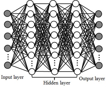
Auto-encoders can automatically learn features from unlabeled data and give feature description better than original data. The process of auto-encoder is to use auto-encoder to find implicit features from input data and make fusion rules through implicit features. Auto-encoder is a neural network which contains the hidden layer. When the number of neurons in the hidden layer is less than that in the input layer, auto-encoder network model can play a role in compressing data. If there are a large number of neurons in the hidden layer, neurons in the hidden layer can transform into the output of the output layer. If the output number in the output layer is the same with the input number in the input layer, its output is considered equivalent to its input.
Auto-encoder is a kind of symmetric multi-layer neural networks, as shown in Fig. 1. It encoded input data through the hidden layer, reconstructed input data by means of the hidden layer, minimized the reconstruction error and obtained the optimal hidden layer expression. Regarding the collected vibration data of the rolling bearing, it was reconstructed as data set , . Namely, sets of data with a length of were selected as experimental data. The input matrix which made up of these vibration data sets was .
Firstly, a multi-layer neural network including the input layer, the hidden layer and the output layer was established. Sigmoid function was selected as the activation function of neurons. The unlabeled input matrix was expected to learn the features of the hidden layer. Input data was reconstructed as output data to highlight the features of original data.
This paper used the sparse auto-encoder with unsupervised feature learning to complete the initialization of the deep neural network, then applied the sparse representation learned by encoder to train the neural network classifier and completed the training and tiny adjustment of the whole deep neural network. For the encoder, the hidden layer was just the extracted feature layer. The expression of the hidden layer was the function which took connection weight value and deviation value as parameters. Therefore, the deep neural network could be initialized according to the parameters of encoder and concise and effective feature expressions of labeled data could be extracted after the optimized was obtained. To obtain better sparse expression and embody the good noise tolerance of sparse automatic coding algorithm, denoising encoding could be added based on sparse encoding and denoising sparse automatic encoder extracting more effective features of data was obtained through training.
The number of neurons in the hidden layer in the deep neural network model might be more important than feature learning algorithm and model depth. Therefore, this paper only studied the deep neural network realized by one-layer sparse auto-encoder. The whole training process of the deep neural network was shown in Fig. 2.
Fig. 2Prediction process of the deep neural network
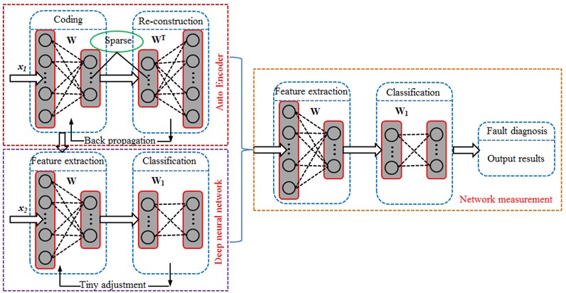
Main description was divided into 3 steps.
1) Used the vibration data of the unlabeled bearing to train sparse auto-encoder.
2) After the encoding of the above encoder, the unlabeled original data would become the labeled data . The labeled vibration data of the bearing was used to train the deep neural network and conduct supervision and classification.
3) Used dataset to measure network performance.
3. Intelligent fault diagnosis of bearings based on several kinds of network models
3.1. Acquisition of experimental data
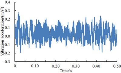
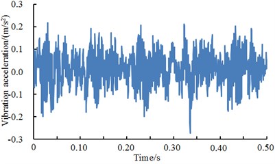
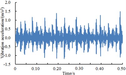
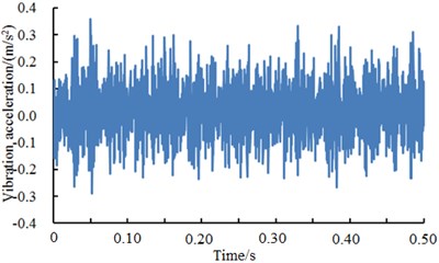
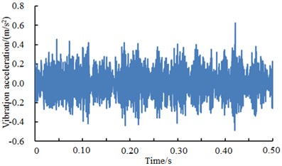
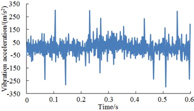
In order to test the fault of the bearing, the experimental system of the fault diagnosis for the bearing is built [26]. In the experiment, a deep groove ball bearing of 6205-2RS type was selected as the rolling element, where the rotation speed was 1772 r/min. Sampling frequency was 12000 Hz, and motor load was 0.746 kW. Firstly, the bearing was in a normal state. The vibration accelerations of the experimental system at different positions were tested. The result was shown in Fig. 3. As shown from the figure, the vibration acceleration of driver end was basically consistent with that of fan end. They fluctuated around 0. The maximum values were no more than 0.3 m/s2 while the minimum values were no less than –0.3 m/s2. In addition, vibration accelerations at different positions presented weak periodicity. The vibration acceleration of driver end showed an obvious valley value around 0.35 s. The vibration acceleration was close to 0.3 m/s2, which was probably caused by the structural resonance of driver end.
Fig. 3Accelerations of different positions under normal working conditions

a) Driver end
b) Fan end
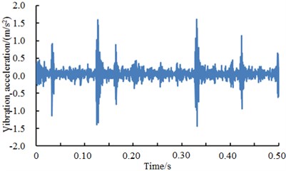
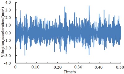
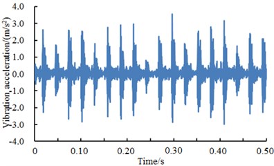
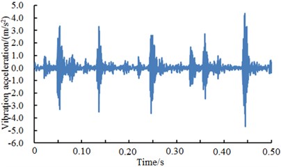
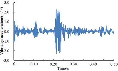
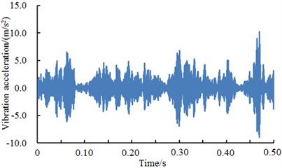
The bearing of driver end was selected as the researched object. Vibration signals with a normal state, an inner ring fault, an outer ring fault and a rolling element fault state were selected as samples. The vibration signals of the rolling bearing under four kinds of conditions are shown in Fig. 4. When inner ring and outer ring of bearings had faults, vibration acceleration was obviously larger than that in a normal state. When the rolling element had faults, the vibration signals of the bearing only reduced the amplitude and there were small changes in value. In addition, it could also be seen from Fig. 4 that the vibration signals of the bearing under various conditions presented periodicity. The periodicity was more obvious when inner ring and outer ring of bearings had faults. Based on the vibration acceleration, the fault type of inner ring and outer ring can be obviously recognized from four kinds of conditions in Fig. 4 because the acceleration had obvious periodicity and peak, while the normal state and the rolling element damage cannot be recognized from four kinds of conditions in Fig. 4 only based on the vibration acceleration. As a result, it was necessary to adopt the deep neural network to recognize the fault of four kinds of conditions.
Fig. 4A comparison of vibration signals of the bearing with different faults
a) Normal state

b) inner ring damage

c) Outer ring damage

d) Rolling element damage
3.2. Comparisons of fault diagnosis based different algorithms
In fact, vibration signals measured at each observation point was not a single signal component. It was made up of different frequency components. The fault signal of the bearing under laboratory conditions was smaller than the vibration signal of the bearing itself. Therefore, only the natural characteristics of the bearing could be seen from time-domain signals. To accurately judge the fault status of the bearing, it was necessary to further extract and analyze the features of vibration signals. The extracted feature vectors were taken as the input of neural networks to train networks. As a result, feature values which were very sensitive to the change of work status should be selected in the case of extracting feature vectors to better train neural networks. Commonly-used feature vectors included two types, namely dimensional and non-dimensional. Dimensional feature vectors could well reflect fault positions and specifically show the degree of faults. Compared with dimensional feature vectors, non-dimensional feature vectors were not closely related to fault mechanism, but they could represent the work status of systems. According to different sensitive degrees to various work conditions and difficulties of extraction, the several kinds of feature vectors were selected for feature extraction. A was mean value, B was skewness factor; C stood for Kurtosis factor; D was Kurtosis index; E was margin factor; F was skewness index; G was Kurtosis; H was spectrum center; I was spectrum variance; J was harmonic factor; K was the dot pitch of spectrum origin. Computational results of these features were shown in Table 1. According to the computational process in Fig. 2, the number of neurons in the input layer was 20; the number of neurons in the hidden layer was 10; the activation function of neurons was sigma function. The training algorithm of the model was back propagation algorithm. Among them, the 500 groups were used as training samples, and the other 1500 groups were used as test samples. The target error was 0.1. The final training error was shown in Fig. 5. It could be found from Fig. 5 that the training error of the deep neural network was close to the target value when the number of training iterations was 260. The computational result was reliable.
Table 1Main feature parameters under 4 kinds of different work conditions
Condition | A | B | C | D | E | F | G | H | I | J | K |
Normal state | 0.09 | 0.7 | 2.7 | 0.12 | 9.7 | 0.04 | 0.05 | 1168 | 58651 | 22.1 | 11054 |
Inner ring damage | 0.02 | –0.46 | 7.0 | 0.37 | 12.8 | –0.04 | 0.12 | 1339 | 48902 | 7.5 | 18444 |
Outer ring damage | 0.002 | –0.13 | 1.4 | 0.98 | 7.6 | –0.04 | 0.84 | 1359 | 40896 | 3.6 | 21106 |
Rolling element damage | 0.03 | 0.07 | 3.2 | 0.64 | 13.8 | 0.01 | 0.61 | 1513 | 67535 | 8.2 | 13236 |
Fig. 5Training error of the deep neural network
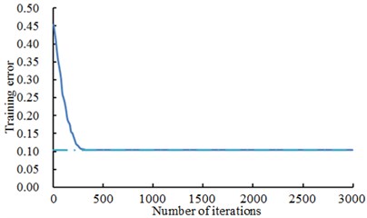
Fig. 6Distribution of the first two principal elements of the rolling bearing
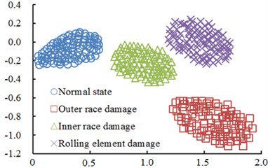
Principal component analysis was used to deal with the original feature set of the bearing and reduce the dimension of feature space. Two-dimensional features correlated with original feature space most were chosen from features after dimension reduction to describe bearing data, as shown in Fig. 6. In the figure, samples of various kinds of work conditions had linear separability. Additionally, various kinds of samples had high aggregation. The aggregation of outer ring fault samples was the poorest.
To further verify the effectiveness of the deep neural network after parameter selection, a comparison between BP neural network (BPNN), genetic algorithm neural network (GANN) and particle swarm optimization neural network (PSONN) was made. The condition of terminating training process of neural network adopted the largest number of iterations and training error. The largest number of iterations in BP neural network was 3000. The largest number of iterations in PSO neural network was 520. The largest number of iterations in GA neural network was 700. Critical error was 0.1. Fig. 7 was a comparison of error convergences of training errors of 4 kinds of neural network models in a training process.
Fig. 7A comparison of training errors of 4 kinds of neural networks
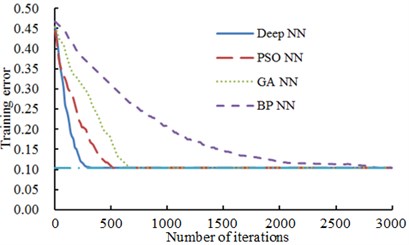
As shown from Fig. 7, the error convergence values of BPNN, GANN and PSONN were 0.287, 0.108 and 0.104 respectively when the number of iterations was 700. Their error convergence values were more than the critical error 0.1. Additionally, BP neural network converged to the critical error 0.1 when the number of iterations was 3000. When the number of iterations was 260, the training error of the deep neural network had converged to 0.099, which was lower than the critical error and completed the training process. When the number of iterations was 520, PSONN converged to 0.104 while GANN converged to 0.20 at this time. Therefore, the deep neural network algorithm showed better training features in the training process of neural network. To avoid randomness, training was repeated 50 times to obtain the average training result of 4 kinds of models, as shown in Table 2.
Table 2A comparison of average training results of 4 kinds of neural networks
Network model | Training error | Number of iterations | Time/s |
BPNN | 0.112 | 2861 | 7.1 |
GANN | 0.108 | 700 | 52.9 |
PSONN | 0.104 | 520 | 5.5 |
Deep NN | 0.099 | 260 | 3.5 |
As shown in Table 2, the training process of BP neural network had a large number of iterations and spent much time, but reached high model precision through small model complexity. GANN adopted large-scale population training and needed global optimization. Therefore, it was very time-consuming. In addition, model precision and complexity were not ideal. PSONN took less time. At present, published reports showed that the prediction accuracy of PSONN was higher than that of BPNN, but model complexity of PSONN is about 3 times that of BPNN. In very short training time, the deep neural network obtained the neural network model with the smallest training error and complexity by virtue of a relatively small number of iterations. Network models obtained by 4 kinds of training were used to classify and diagnose test samples. The obtained diagnosis result was shown in Table 3.
Table 3A comparison of diagnosis results of 4 kinds of neural networks
Network model | Diagnosis accuracy rates (%) | ||
Maximum value | Minimum value | Average value | |
BPNN | 92.31 | 57.78 | 85.27 |
GANN | 94.52 | 41.00 | 76.60 |
PSONN | 95.46 | 57.71 | 88.47 |
Deep NN | 99.78 | 90.67 | 96.64 |
As shown from Table 3, the average test accuracy rate of the deep neural network was the highest, namely 94.04 %, and increased by 11.37 %, 20.04 % and 8.17 % respectively compared with that of BPNN, GANN and PSONN. In many experiments, the minimum values of accuracy rates obtained by BPNN, GANN and PSONN were around 50 %. The accuracy rate of GANN was 41 %. About the reason, 3 kinds of neural networks had the problem of local extremum in their training processes. Training errors could not further converge and learning of network models was inadequate, which led to the invalidity of diagnosis. The lowest accuracy rate of the deep neural network was 90.67 %, which was higher than that of other three kinds of neural network models.
3.3. Stability of the deep neural network
In order to show stability of the method proposed in this paper, we compared the computational results of this method with the related work when the other conditions are consistent.
Based on the neural network method, Reference [27] proposed an intelligent fault diagnosis method and researched the influences brought by different sample numbers and percentages of neutral network training data to the diagnosis accuracy rate. The computational method proposed by reference [27] shows obvious superiorities in accuracy rate compared with the traditional computational methods. Therefore, it is fair to conclude that the fault diagnosis method mentioned in reference [27] is a relatively advanced method at present. The same problem was researched by the method proposed in this paper. Research results are compared with results of reference [27]. Comparison results are shown in Fig. 8 and Fig. 9.
It is shown in Fig. 8 that the diagnosis accuracy rate increased with the sample numbers increase when the percentage of neutral network training data was 10 %. When the sample numbers were 500, the diagnosis accuracy rate of the method proposed by this paper was 0.865, while the result was 0.817 for reference [27]. When the sample numbers were 1000, the computational result for the method proposed in this paper was 0.959, while the result for reference [27] was 0.946. With continuous increase of sample numbers, reference [27] showed higher diagnosis accuracy rate. The method proposed by this paper showed obvious superiorities for small sample numbers. In case of large sample numbers, the computational accuracy rate of the method proposed by this paper still approached that of reference [27]. In addition, in actual engineering application, such huge sample numbers will not be used for the diagnosis very commonly. Therefore, the diagnosis method proposed by this paper is of greater significance in actual engineering applications.
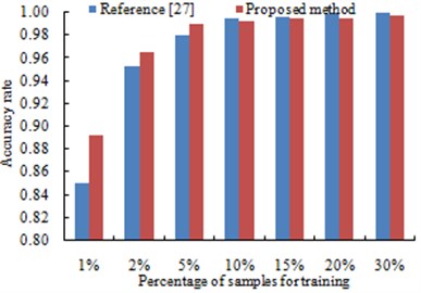
In addition, in order to compare the method with reference [27], the influences brought by different training data percentages to the diagnosis accuracy rate in the neutral network training were researched under the constant sample numbers of 20000, as shown in Fig. 10. It is shown in Fig. 9 that under the percentage of 1 %, the diagnosis accuracy rate of the method proposed by this paper was 0.892, and the result for reference [27] was 0.850. Under the percentage of 2 %, the diagnosis accuracy rate for method in this paper was 0.965, and the result for reference [27] was 0.952. With continuous increase of the percentage, the diagnosis accuracy rate of the method proposed by this paper was lower than that of reference [27], but the accuracy rate of both the methods were still very close. As well, large numbers of samples are not commonly used in actual engineering for diagnosis. Therefore, in diagnosis with a small sample numbers, the method proposed by this paper is obviously superior.
Fig. 8Diagnosis results using different group numbers
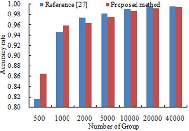
Fig. 9Diagnosis results using different percentages of samples
4. Influence of fault levels and excitation loads of bearings on diagnosis accuracy rates
From the above analysis, it showed that the deep neural network had obvious advantages in stability and diagnosis accuracy compared with traditional neural network algorithms and the latest reported algorithms. Therefore, the deep neural network was applied to the experimental system to detect the faults of different excitation loads and fault levels.
4.1. Fault diagnosis of different fault levels
The no-load condition of the motor remained unchanged. Namely, the fault diagnosis rate of different fault levels of bearings using the deep neural network was studied when the test system bore consistent excitation loads, as shown in Fig. 10, Fig. 11 and Fig. 12.
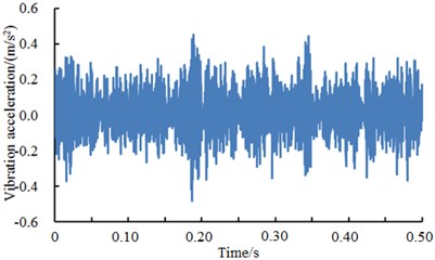
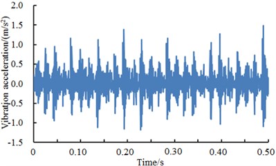
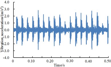
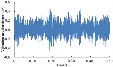
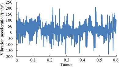
Fig. 10 presented the vibration accelerations of inner ring with a fault diameter of 7 mm, 14 mm and 21 mm and 28 mm respectively. It could be seen from the figure that vibration accelerations presented the periodicity when the fault diameter of inner ring was less than 28 mm. Aimed at different fault diameters, vibration periodicity was different. In particular, the vibration acceleration of the bearing showed more obvious periodicity and peak value when the fault diameter of the bearing was 14 mm. When the fault diameter was 28 mm, the vibration acceleration of the bearing obviously increased. In addition, peak values were more intensive and periodicity became weaker. The fault type of the bearing could not be recognized only according to vibration signals. It could be noticed from the figure that different faults of bearings showed obvious differences in vibration acceleration and fault features. Therefore, the deep neural network could be used to recognize the fault of different fault levels of bearings. The result was shown in Table 4.
Table 4Fault diagnosis rate of different faults of inner ring
Fault type | Diagnosis accuracy rates (%) | ||
Maximum value | Minimum value | Average value | |
7 mm | 99.78 | 90.67 | 96.64 |
14 mm | 99.96 | 95.12 | 98.20 |
21 mm | 99.82 | 93.22 | 97.33 |
28 mm | 97.31 | 89.09 | 94.41 |
As shown from Table 4, the average diagnosis accuracy rates using deep neural network were higher. The minimum value was 94.41 %. The maximum value was 98.20 %. For different fault levels, diagnosis accuracy rates were different mainly because the fault features of vibration signals were different obviously. As shown in Fig. 10, vibration features were particularly obvious when the fault diameter was 14 mm. Therefore, diagnosis accuracy rates were very high when the deep neural network was used for fault diagnosis. When the fault diameter was 28 mm, fault features were not obvious. Therefore, the fault diagnosis rates using the deep neural network were not very high. However, the fault diagnosis rate 94.41 % was very high compared with the reported algorithms. The deep neural network still had obvious advantages.
Fig. 10A comparison of vibration signals of different fault levels of inner ring
a) Inner ring 7 mm
b) Inner ring 14 mm
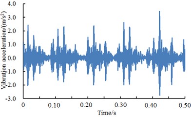
c) Inner ring 21 mm
d) Inner ring 28 mm
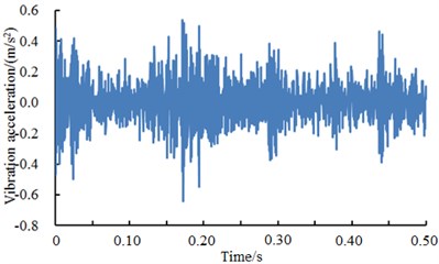
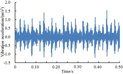
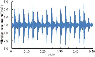
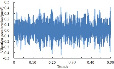
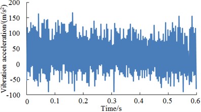
Fig. 11 showed the vibration accelerations of bearing outer ring when the fault diameter was 7 mm, 14 mm, 21 mm and 28 mm. It could be seen from the figure that vibration signals of the bearing had obvious periodicity and peak values when the fault diameter was 7 mm, 21 mm and 28 mm. However, periodicity was not obvious when the fault diameter was 14 mm. The fault type of the bearing could not be recognized only according to vibration signals. As shown from the figure, different fault levels of bearings showed obvious differences in vibration acceleration and fault features. Therefore, the deep neural network could be used to recognize the fault of different fault levels of bearings. The result was shown in Table 5.
Table 5Fault diagnosis rates of different fault levels of outer ring
Fault type | Diagnosis accuracy rates (%) | ||
Maximum value | Minimum value | Average value | |
7 mm | 99.16 | 95.11 | 96.77 |
14 mm | 96.17 | 90.02 | 92.18 |
21 mm | 99.66 | 96.14 | 97.70 |
28 mm | 97.57 | 92.35 | 94.91 |
As shown from Table 5, the average diagnosis accuracy rates using deep neural network were higher. The minimum value was 92.18 %. The maximum value was 97.70 %. For different fault types, diagnosis accuracy rates were different mainly because the fault features of vibration signals were different obviously. As shown in Fig. 11, vibration features were particularly obvious when the fault diameter was 21 mm. Therefore, diagnosis accuracy rates were very high when the deep neural network was used for fault diagnosis. When the fault diameter was 14 mm, fault features were not obvious. However, fault features were not obvious when the fault diameter was 14 mm. Therefore, the fault diagnosis rate using the deep neural network was not very high. However, the fault diagnosis rate 92.18 % was very high compared with reported algorithms. The deep neural network still had obvious advantages.
Fig. 11A comparison of vibration signals of different fault levels of outer ring
a) Outer ring 7 mm
b) Outer ring 14 mm
c) Outer ring 21 mm
d) Outer ring 28 mm
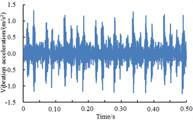
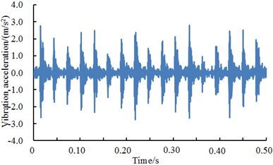
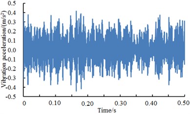
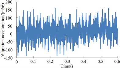
Fig. 12 showed the vibration accelerations of bearing rolling element when the fault diameter was 7 mm, 14 mm, 21 mm and 28 mm. It could be seen from the figure that vibration accelerations of all faults showed no obvious periodicity and peak values when the fault diameter was less than 28 mm. However, periodicity and peak values were obvious when the fault diameter was 28 mm. The fault type of bearings could not be recognized only according to vibration signals. Therefore, the deep neural network could be used to recognize the fault of different fault levels of bearings. The result was shown in Table 6.
Table 6Fault diagnosis rates of different fault levels of the rolling element
Fault type | Diagnosis accuracy rates (%) | ||
Maximum value | Minimum value | Average value | |
7 mm | 96.02 | 89.99 | 91.06 |
14 mm | 95.37 | 90.22 | 91.25 |
21 mm | 97.09 | 90.88 | 93.44 |
28 mm | 98.22 | 92.38 | 94.16 |
As shown from Table 6, the average diagnosis accuracy rates using the deep neural network were higher. The minimum value was 91.06 %. The maximum value was 94.16 %. For different fault types, diagnosis accuracy rates were different mainly because the fault features of vibration signals were different obviously. As shown in Fig. 12, vibration features were particularly obvious when the fault diameter was 28 mm. Therefore, diagnosis accuracy rates were very high when the deep neural network was used for fault diagnosis. When the fault diameter was not 28 mm, fault features were not obvious. However, the fault diagnosis rate 91.06 % was very high compared with reported algorithms. The deep neural network still had obvious advantages.
Fig. 12A comparison of vibration signals of different fault levels of the rolling element
a) Rolling element 7 mm
b) Rolling element 14 mm
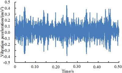
c) Rolling element 21 mm
d) Rolling element 28 mm
4.2. Fault diagnosis of different excitation loads
The fault diameter of 7 mm remained unchanged to study the fault diagnosis rate of bearings with different excitation loads using the deep neural network, as shown in Fig. 13, Fig. 14 and Fig. 15.
Fig. 13 showed vibration accelerations of inner ring when excitation loads were 0 HP, 1 HP, 2 HP and 3 HP. It could be seen from the figure that vibration accelerations of inner ring had obvious peak values and periodic features under different excitation loads. In addition, vibration accelerations of inner ring presented similar periodicity and amplitude under different excitation loads. However, fault type could not be recognized only according to vibration signals because features under each excitation load were so similar. Therefore, the deep neural network was used to diagnose the fault of various kinds of work conditions. The result was shown in Table 7.
Table 7Fault diagnosis rates of inner ring under different excitation loads
Fault type | Diagnosis accuracy rates (%) | ||
Maximum value | Minimum value | Average value | |
0 HP | 99.45 | 94.77 | 96.88 |
1 HP | 99.56 | 95.21 | 97.23 |
2 HP | 99.14 | 95.09 | 97.04 |
3 HP | 99.68 | 95.90 | 97.99 |
As shown from Table 7, diagnosis rates under different fault types were very high. The minimum value was 96.88 % while the maximum value was 97.99 %. As vibration accelerations of bearings under each fault had obvious features, the deep neural network could be used to effectively extract the fault features of bearings. Compared with the analysis in Section 4.1, fault diagnosis rates obviously increased.
Fig. 13A comparison of vibration signals of inner ring under different excitation loads
a) Inner ring 0 HP
b) Inner ring 1 HP
c) Inner ring 2 HP
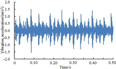
d) Inner ring 3 HP
Fig. 14 showed vibration accelerations of outer ring when excitation loads were 0 HP, 1 HP, 2 HP and 3 HP. It could be seen from the figure that vibration accelerations of outer ring had obvious peak values and periodic features under different excitation loads. In addition, vibration accelerations of outer ring presented similar periodicity and amplitude under different excitation loads. However, fault type could not be recognized only according to vibration signals because features of each excitation load were so similar. Therefore, the deep neural network was used to diagnose the fault of various kinds of work conditions. The result was shown in Table 8.
Table 8Fault diagnosis rates of outer ring under different excitation loads
Fault type | Diagnosis accuracy rates (%) | ||
Maximum value | Minimum value | Average value | |
0 HP | 99.21 | 94.67 | 96.17 |
1 HP | 99.50 | 95.13 | 96.60 |
2 HP | 99.81 | 96.20 | 97.45 |
3 HP | 99.34 | 94.90 | 96.51 |
As shown from Table 8, diagnosis rates under different fault types were very high. The minimum value was 96.17 % while the maximum value was 97.45 %. As vibration accelerations of bearings of each fault showed obvious features, the deep neural network could be used to effectively extract the fault features of the bearing.
Fig. 15 showed vibration accelerations of the rolling element when excitation loads were 0 HP, 1 HP, 2 HP and 3 HP. It could be seen from the figure that vibration accelerations of the rolling element had no obvious peak values and periodic features under different excitation loads. However, fault type could not be recognized only according to vibration signals. Therefore, the deep neural network was used to diagnose the fault of various kinds of work conditions. The result was shown in Table 9.
Fig. 14A comparison of vibration signals of outer ring under different excitation loads

a) Outer ring 0 HP
b) Outer ring 1 HP
c) Outer ring 2 HP
d) Outer ring 3 HP
Table 9Fault diagnosis rates of the rolling element under different excitation loads
Fault type | Diagnosis accuracy (%) | ||
Maximum value | Minimum value | Average value | |
0 HP | 96.56 | 90.08 | 92.32 |
1 HP | 95.12 | 89.29 | 91.09 |
2 HP | 95.01 | 89.38 | 91.36 |
3 HP | 96.77 | 91.27 | 93.31 |
As shown from Table 9, diagnosis rates under different fault types had some gaps. The minimum value was 91.09 % while the maximum value was 93.31 %. Compared with faults of inner ring and outer ring, diagnosis rates had an obvious decrease mainly because features of vibration acceleration of the rolling element fault were not obvious. In addition, the amplitude of vibration acceleration of the rolling element was obviously less than that of inner ring and outer ring faults.
Fig. 15A comparison of vibration signals of the rolling element under different excitation loads
a) Rolling element 0 HP
b) Rolling element 1 HP
c) Rolling element 2 HP
d) Rolling element 3 HP
5. Application of deep neural networks in complex machinery.
At present, wind turbines have been widely applied. There were a lot of reasons for the fault and vibration of wind turbines. The source of faults of wind turbines was gearbox. In the meanwhile, gearbox faults also had a great influence on the whole wind turbine. Related studies and tests on wind turbines have been widely published. However, the published accuracy of fault diagnosis was not high. This paper used proposed deep neural network technology to diagnose it again based on the published data [28], selected normal work conditions, slight wear, moderate wear and fracture of teeth as researched objects and analyzed the vibration signals generated by faults so as to help the fault diagnosis of wind turbines. The original signal of four kinds of conditions of wind turbines was shown in Fig. 16. As shown from the original signal in Fig. 16, it could be observed that the gearbox had some differences in vibration signal under four kinds of different status, but it was difficult to recognize fault status and understand correlation of vibration signals. The proposed deep neural networks were used to diagnose the fault of gearbox and compared with results of classical artificial neural networks including BPNN, GANN and PSONN, as shown in Table 10.
Table 10A comparison of diagnosis results of 4 kinds of neural networks
Network model | Diagnosis accuracy rates (%) | ||
Maximum value | Minimum value | Average value | |
BPNN | 91.21 | 55.64 | 81.32 |
GANN | 92.12 | 43.25 | 77.68 |
PSONN | 94.36 | 61.20 | 89.22 |
Deep NN | 98.91 | 91.28 | 96.42 |
As shown from Table 10, the maximum and minimum values using deep neural networks for diagnosis were 91.28 % and 98.91 % respectively. The average result of diagnosis was 96.42 %. The maximum and minimum values of computational results of other three kinds of classical neural networks presented large differences and poor stability. Meantime, average diagnosis results were low, which fully indicated that deep neural networks proposed in this paper had extensive adaptability in complex machinery.
Fig. 164 kinds of fault conditions of the gearbox
a) Normal work condition
b) Slight wear of tooth surface
c) Moderate wear of tooth surface
d) Fracture of teeth
6. Conclusions
1) The vibration acceleration of driver end in the test system was basically consistent with that of fan end. They fluctuated around 0. The maximum values were not more than 0.3 m/s2 while the minimum values were not less than –0.3 m/s2. In addition, vibration accelerations at different positions presented weak periodicity.
2) The deep neural network was used to recognize the diagnosis rate of the bearing with four kinds of conditions and compared with traditional BPNN, GANN and PSONN. Results showed that the diagnosis accuracy and convergence rate of the deep neural network were obviously higher than those of other models.
3) Fault diagnosis rates of the deep neural network under different sample sizes and training sample proportions were studied to compare with the latest reported methods. Results showed that the deep neural network showed higher fault diagnosis rates under small sample sizes and low percentages. Fault diagnosis presented a good stability.
4) Vibration accelerations of the bearing with different fault diameters and excitation loads were extracted. Vibration accelerations did not present obvious periodicity and features. The deep neural network was used to recognize these faults. Diagnosis accuracy rates were very high. In particular, the fault diagnosis rate was 98 % when signal features of vibration acceleration were very obvious, which indicated that using deep neural network was effective in diagnosing and recognizing different types of faults.
5) The proposed deep neural networks were used to diagnose the fault of gearbox of wind turbines and compared with results of classical artificial neural networks including BPNN, GANN and PSONN. The maximum and minimum diagnosis accuracy rates of other three kinds of classical neural networks presented large differences and poor stability. Meantime, average diagnosis results were low, which fully indicated that deep neural networks proposed in this paper had extensive adaptability in complex machinery.
References
-
Randall R. B., Antoni J. Rolling element bearing diagnostics – a tutorial. Mechanical Systems and Signal Processing, Vol. 25, Issue 2, 2011, p. 485-520.
-
Harris T. A., Kotzalas M. N. Rolling Bearing Analysis Essential Concepts of Bearing Technology. CRC Press Inc., New York, 2007.
-
Chen K. J. Study on Ball Bearing Fault Diagnosis Based on Vibration Signals. Xidian University, Xi’an, 2011.
-
Mahanty R. N., Gupta P. B. D. Application of RBF neural network to fault classification and location in transmission lines. IEE Proceedings of Generation, Transmission and Distribution, Vol. 151, Issue 2, 2004, p. 201-212.
-
Kankar P. K., Sharma S. C., Harsha S. P. Vibration-based fault diagnosis of a rotor bearing system using artificial neural network and support vector machine. International Journal of Modelling, Identification and Control, Vol. 15, Issue 3, 2012, p. 185-198.
-
Ahmed R., El Sayed M., Gadsden S. A., et al. Automotive internal-combustion-engine fault detection and classification using artificial neural network techniques. IEEE Transactions on Vehicular Technology, Vol. 64, Issue 1, 2015, p. 21-33.
-
Baklacioglu T., Turan O., Aydin H. Dynamic modeling of exergy efficiency of turboprop engine components using hybrid genetic algorithm-artificial neural networks. Energy, Vol. 86, 2015, p. 709-721.
-
Wei X. T., Pan H. X., Ma Q. F. Application of particle swarm optimization based on neural network to fault diagnosis. Journal of Vibration, Measurement and Diagnosis, Vol. 26, Issue 2, 2006, p. 133-137.
-
Yang X. S. Firefly algorithm for multimodal optimization. Lecture Notes in Computer Science, Vol. 5972, 2009, p. 169-178.
-
Samanta B., Al Balushi K.-R. Artificial neural network based fault diagnostics of rolling element bearings using time-domain features. Mechanical systems and signal processing, Vol. 17, Issue 2, 2003, p. 317-328.
-
Martins J. F., Pires V. F., Pires A. J. Unsupervised neural-network-based algorithm for an on-line diagnosis of three-phase induction motor stator fault. IEEE Transactions on Industrial Electronics, Vol. 54, Issue 1, 2007, p. 259-264.
-
Cheriyadat A. M. Unsupervised feature learning for aerial scene classification. IEEE Transactions on Geoscience and Remote Sensing, Vol. 52, Issue 1, 2014, p. 439-451.
-
Erhan D., Bengio Y., Courville A., et al. Why does unsupervised pre-training help deep learning? Journal of Machine Learning Research, Vol. 11, 2010, p. 625-660.
-
Lee H., Pham P., Largman Y., et al. Unsupervised feature learning for audio classification using convolutional deep belief networks. Advances in Neural Information Processing Systems, 2009, p. 1096-1104.
-
Hinton G. E., Salakhutdinov R. R. Reducing the dimensionality of data with neural networks. Science, Vol. 313, Issue 5786, 2006, p. 504-507.
-
Ciregan D., Meier U., Schmidhuber J. Multi-column deep neural networks for image classification. IEEE Conference on Computer Vision and Pattern Recognition (CVPR), 2012, p. 3642-3649.
-
Simonyan K., Zisserman A. Very deep convolutional networks for large-scale image recognition. Computer Vision and Pattern Recognition, 2015.
-
Tang J., Deng C., Huang G. B., et al. Compressed-domain ship detection on spaceborne optical image using deep neural network and extreme learning machine. IEEE Transactions on Geoscience and Remote Sensing, Vol. 53, Issue 3, 2015, p. 1174-1185.
-
Hinton G., Deng L., Yu D., et al. Deep neural networks for acoustic modeling in speech recognition: The shared views of four research groups. IEEE Signal Processing Magazine, Vol. 29, Issue 6, 2012, p. 82-97.
-
Dahl G. E., Yu D., Deng L., et al. Context-dependent pre-trained deep neural networks for large-vocabulary speech recognition. IEEE Transactions on Audio, Speech, and Language Processing, Vol. 20, Issue 1, 2012, p. 30-42.
-
Xu Y., Du J., Dai L. R. An experimental study on speech enhancement based on deep neural networks. IEEE Signal Processing Letters, Vol. 21, Issue 1, 2014, p. 65-68.
-
Coates A., Ng A. Y. The importance of encoding versus training with sparse coding and vector quantization. Proceedings of the 28th International Conference on Machine Learning (ICML-11), 2011, p. 921-928.
-
Lyons J., Dehzangi A., Heffernan R., et al. Predicting backbone Cα angles and dihedrals from protein sequences by stacked sparse auto-encoder deep neural network. Journal of Computational Chemistry, Vol. 35, Issue 28, 2014, p. 2040-2046.
-
Su S. Z., Liu Z. H., Xu S. P., et al. Sparse auto-encoder based feature learning for human body detection in depth image. Signal Processing, Vol. 112, 2015, p. 43-52.
-
Bengio Y., Lambin P., Popovici D. Greedy layer wise training of deep networks. Advances in Neural Information Processing Systems 19, Vancouver, Canada, 2007, p. 153-160.
-
Case Western reserve university Bearing Data Center. Bearing Data Center Fault Test Data, http://www.eecs.case.edu/laboratory/bearing.
-
Lei Y. G., Jia F., Xing S. B., Ding S. X. An intelligent fault diagnosis method using unsupervised feature learning towards mechanical big data. IEEE Transactions on Industrial Electronics, Vol. 63, Issue 5, 2016, p. 3137-3147.
-
Lin Y. H. Study on Wind Turbine Fault Diagnosis Decision System Based on Wavelet Analysis and Neural Network Method. Xi’an University of Technology, Xi’an, 2014.
Cited by
About this article

The authors are very grateful for the financial support from the National Natural Science Foundation of China (Nos. 61502129 and 61163016), the Natural Science Foundation of Zhejiang Province of China (No. LQ16F020004), and the University Scientific Research Projects of Ningxia Province of China (No. NGY2015161).
