Bifurcation and chaos characteristic analysis of spur micro-segment gear pair

2.1. Mathematical representation of dynamic model for micro-segment gear pair

The mechanical model is shown in Fig. 1. Two gears are combined with supporting shafts, which are regarded as rigid bodies with large support stiffness. The pinion and gear are represented by their base circles with radius $r_{bp}$ and $r_{bg}$, respectively. The equations of motion can be expressed as:

where, $I_p$ and $I_g$ are polar mass moments of inertia. $m_p$ and $m_g$ are masses. $K\left(t\right)$ is time-varying mesh stiffness. $c_m=2\zeta \sqrt{k_m/\left(1/m_p+1/m_g\right)}$ is viscous damping. $D\left(t\right)$ is time-varying profile deviation of micro-segment gear comparing with involute gear. The static transmission error $e\left(t\right)$ is regarded as internal excitation which can be expressed in a Fourier series in the form:

Fig. 1a) Snap shot of contact pattern (at t= 0) of a spur micro-segment gear pair; b) the non-linear dynamic model

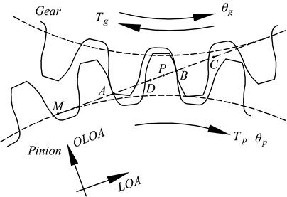
a)

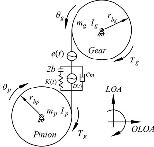
b)

The external excitations $T_P$ and $T_g$ are acting on the pinion and gear which can be decomposed into average torque $T_m$ and fluctuating external torque excitation $T\left(t\right)$. To simplify the calculation, the fluctuation of output torque is neglected, i.e. $T_g=\mathrm{}{T}_{gm}$ and input torque can be expressed via Fourier series as:

The backlash function $h$ is usually calculated by:

By employing a composite co-ordinate:

Eq. (1) can be re-formed as:

with:

where $m_e$ is the equivalent mass. $F_m$ is average force and $F_p\left(t\right)$ is the fluctuating force related to external torque excitation. $F_e\left(t\right)$ is the fluctuating force related to internal displacement excitation.

2.2. Two important parameters in dynamic model $\left(\mathit{K}\left(\mathit{t}\right),\mathit{D}\left(\mathit{t}\right)\right)$

The main difference between proposed dynamic model and the traditional SDOF is embodied in two important parameters $K\left(t\right)$ and $D\left(t\right)$.

2.2.1. Time-varying mesh stiffness $\mathit{K}\left(\mathit{t}\right)$

The time-varying mesh stiffness greatly affects the dynamics of gear system. According to the available literature, the mesh stiffness is usually simplified or calculated by the empirical equations. These methods are often based on the classical theory of elasticity and numerical approaches. However, it is considered to be unsuitable to use these methods on the dynamic research of micro-segment gear due to the special profile. Therefore, the finite element method is utilized to calculate the mesh stiffness. With the design parameters of micro-segment gears listed in table 1, the 3D finite element model for a pair of tooth of micro-segment gear is shown in Fig. 2.

Fig. 2The entity model of micro-segment gear

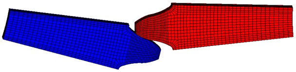
The 3D finite element model contains about 9840 elements and the tooth thickness in mesh model is set to 1mm. Four end faces and one cylindrical face are fixed, and the other cylindrical face is defined as the loading surface. Since the gear meshing is a nonlinear process, the contact surfaces are defined as nonlinear contacting to get a more realistic result.

Table 1Common design parameters of the spur gear pairs

Parameter	Pinion/Gear
Number of teeth	45
Transverse module (mm)	2
Width (mm)	20
Mass (kg)	0.885
Moments of inertia (kg$\bullet$m2)	9.988e-004
Density (kg/m3)	9860
Elasticity modulus (GPa)	205
Poisson ratio	0.3

In the meshing process of a gear set with a contact ratio $\epsilon \mathrm{}$lower than 2, we can conceptually consider that there are always two pairs of teeth (pair #1 and pair #2) under contact. In Fig. 1(a), the meshing teeth pair with contact point located between point A and point B is defined as pair #1, and the meshing teeth pair with contact point located between point B and point C is defined as pair #2.

Fig. 3The mesh stiffness of micro-segment gear

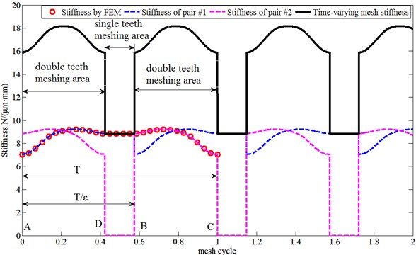
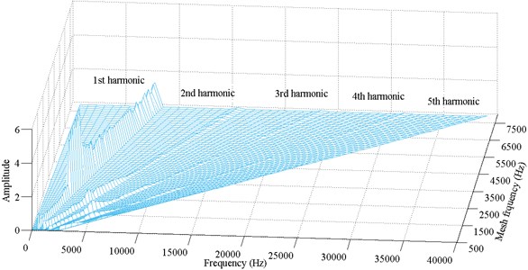
The mesh stiffness for a pair of teeth from A to C, can be calculated by the FEM mentioned above, and can be expressed in the form of Fourier series expansion as follow:

7

$k\left(t\right)=k_m+\sum _{j=1}^8\left(k_{aj}\cos \left(j{w}_{k}t\right)+k_{bj}\mathrm{s}\mathrm{i}\mathrm{n}\left(j{w}_{k}t\right)\right),$

where $k_m$ is average mesh stiffness. $k_{aj}$, $k_{bj}$ are amplitudes of the $j$th order harmonic. $w_k$ is fitting frequency; then we have $T=2\pi /w_k$, here $T$ is the period of the mesh stiffness $k\left(t\right)$ for one pair of teeth, rather than the time-varying mesh stiffness for the gear set. A good fit can be achieved with the first eight orders of the Fourier series, as show in Fig. 3 and fitting parameters are listed in Table 2.

Table 2Fitting parameters of stiffness (Nμm-1 mm-1) and synthetically normal deviation (mm)

$j$	$k_{aj}$	$k_{bj}$	$d_{aj}$	$d_{bj}$
1	–6.541e-1	–2.101e-4	–8.088e-2	1.733e-05
2	–6.419e-1	–2.997e-4	2.627e-2	–3.418e-05
3	–2.142e-1	–1.55e-4	6.399e-3	5.01e-05
4	–6351e-2	–6.556e-05	7.992e-4	–6.465e-05
5	–4.607e-2	–6.824e-05	9.012e-4	7.744e-05
6	1.491e-2	2.454e-06	3.851e-4	–8.812e-05
7	1.028e-2	1.405e-05	1.61e-4	9.64e-05
8	8.566e-3	–7.323e-07	6.113e-4	–0.000102
$k_m$	8.622		/
$d_m$	/		–0.01078

Then, the time-varying mesh stiffness can be obtained by summing the stiffness of pair #1 and pair #2, as show in Fig. 3. According to Fig. 3, it can be found that the frequency of time-varying mesh stiffness function is $\epsilon w_e$, and the piecewise stiffness functions can be expressed as:

8

$k_1\left(t\right)=k_m+\sum _{j=1}^8\left(k_{aj}\cos \left(j{\omega }_k\mathrm{m}\mathrm{o}\mathrm{d}\left(t,\frac{T}{\epsilon }\right)\right)+k_{bj}\sin \left(j{\omega }_k\mathrm{m}\mathrm{o}\mathrm{d}\left(t,\frac{T}{\epsilon }\right)\right)\right),$

9

$k_2\left(t\right)=\left\{\begin{array}{ll}k\left(\mathrm{m}\mathrm{o}\mathrm{d}(t,T)+\frac{T}{\epsilon }\right),& 0\le \mathrm{m}\mathrm{o}\mathrm{d}\left(t,T\right)<\frac{T\epsilon -T}{\epsilon },\\ 0,& \frac{T\epsilon -T}{\epsilon }\le \mathrm{m}\mathrm{o}\mathrm{d}\left(t,T\right)<\frac{T}{\epsilon },\end{array}\right.$
$=\left\{\begin{array}{ll}{k}_m+\sum _{j=1}^8\left(\begin{array}{c}{k}_{aj}\cos \left(j{\omega }_k\left(\mathrm{m}\mathrm{o}\mathrm{d}\left(t,\frac{T}{\epsilon }\right)+\frac{T}{\epsilon }\right)\right)\\ +k_{bj}sin\left(j{\omega }_k\left(\mathrm{m}\mathrm{o}\mathrm{d}(t,\frac{T}{\epsilon })+\frac{T}{\epsilon }\right)\right)\end{array}\right),& 0\le \mathrm{m}\mathrm{o}\mathrm{d}\left(t,T\right)<\frac{T\epsilon -T}{\epsilon },\\ 0,& \frac{T\epsilon -T}{\epsilon }\le \mathrm{m}\mathrm{o}\mathrm{d}\left(t,T\right)<\frac{T}{\epsilon },\end{array}\right.$

10

$k\left(t\right)=k_1\left(t\right)+k_2\left(t\right)$
$=\left\{\begin{array}{ll}k\left(\mathrm{m}\mathrm{o}\mathrm{d}\left(t,\frac{T}{\epsilon }\right)+\frac{T}{\epsilon }\right)+k\left(\mathrm{m}\mathrm{o}\mathrm{d}\left(t,\frac{T}{\epsilon }\right)\right),& 0\le \mathrm{m}\mathrm{o}\mathrm{d}\left(t,\frac{T}{\epsilon }\right)<\frac{T\epsilon -T}{\epsilon },\\ k\left(\mathrm{m}\mathrm{o}\mathrm{d}\left(t,\frac{T}{\epsilon }\right)\right),& \frac{T\epsilon -T}{\epsilon }\le \mathrm{m}\mathrm{o}\mathrm{d}\left(t,\frac{T}{\epsilon }\right)<\frac{T}{\epsilon },\end{array}\right.$
$=\left\{\begin{array}{ll}\begin{array}{c}2k_m+\sum _{j=1}^8\left(\begin{array}{c}{k}_{aj}\cos \left(j{\omega }_k\left(\mathrm{m}\mathrm{o}\mathrm{d}\left(t,\frac{T}{\epsilon }\right)+\frac{T}{\epsilon }\right)\right)\\ +k_{bj}\sin \left(j{\omega }_k\left(\mathrm{m}\mathrm{o}\mathrm{d}\left(t,\frac{T}{\epsilon }\right)+\frac{T}{\epsilon }\right)\right)\end{array}\right)\\ +\sum _{j=1}^8\left(\begin{array}{c}{k}_{aj}\cos \left(j{\omega }_k\mathrm{m}\mathrm{o}\mathrm{d}\left(t,\frac{T}{\epsilon }\right)\right)\\ +k_{bj}\sin \left(j{\omega }_k\mathrm{m}\mathrm{o}\mathrm{d}\left(t,\frac{T}{\epsilon }\right)\right)\end{array}\right),\end{array}& 0\le \text{mod}\left(t,\frac{T}{\epsilon }\right)<\frac{T\epsilon -T}{\epsilon },\\ k_m+\sum _{j=1}^8\left(\begin{array}{c}{k}_{aj}\cos \left(j{\omega }_k\mathrm{m}\mathrm{o}\mathrm{d}\left(t,\frac{T}{\epsilon }\right)\right)\\ +k_{bj}\sin \left(j{\omega }_k\mathrm{m}\mathrm{o}\mathrm{d}\left(t,\frac{T}{\epsilon }\right)\right)\end{array}\right),& \frac{T\epsilon -T}{\epsilon }\le \mathrm{m}\mathrm{o}\mathrm{d}\left(t,\frac{T}{\epsilon }\right)<\frac{T}{\epsilon }.\end{array}\right.$

2.2.2. Time-varying profile deviation $\mathit{D}\left(\mathit{t}\right)$

The normal deviation of micro-segment gear compared with the standard involute profile will be analyzed in this section. In Fig. 4, the geometric models of the single tooth for both micro-segment gear and standard involute gear are established. It is clear that these two profiles are obviously different.

Fig. 4The geometric models for both micro-segment gear and standard involute gear

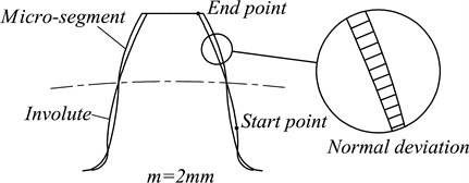
To research the influence of different profiles on the dynamic characteristics of the gear system, the magnitude of deviation should be accurately expressed. In the process of meshing for a pair of teeth, the contact point of the pinion moves from start point to end point and the corresponding point in the gear moves from end point to start point. This process is divided into many small sections in terms of angle, and each micro-angle corresponds to a normal deviation, as show in Fig. 4. Due to the cooperative working of two gears, the displacement excitation of profile deviation $d\left(t\right)\mathrm{}$ should be the normal resultant for both of the gear and pinion body in Fig. 5.

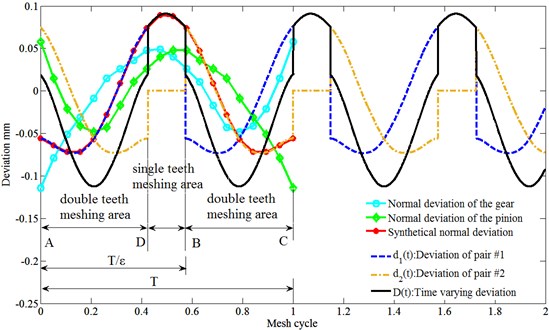
Identical to the time-varying mesh stiffness, the synthetically normal deviation of a pair of teeth also can be expressed as following Fourier series expansion, the fitting parameters are also listed in Table 2:

11

$d\left(t\right)=d_m+\sum _{j=1}^8\left[d_{aj}\mathrm{c}\mathrm{o}\mathrm{s}\left(j{\omega }_{k}t\right)+d_{bj}\mathrm{s}\mathrm{i}\mathrm{n}\left(j{\omega }_{k}t\right)\right],$

where $d_m$ is average deviation of synthetically normal deviation. $d_{aj}$, $d_{bj}$ are amplitudes of the jth order harmonic. The time-varying profile synthetize deviation for the example system is also a piecewise function which can be expressed as follow:

12

$D\left(t\right)=d_1\left(t\right)+d_2\left(t\right)=\left\{\begin{array}{ll}\left(\begin{array}{c}d\left(\text{mod}\left(t,\frac{T}{\epsilon }\right)+\frac{T}{\epsilon }\right)\\ +d\left(\text{mod}\left(t,\frac{T}{\epsilon }\right)\right)\end{array}\right),& 0\le \text{mod}\left(t,\frac{T}{\epsilon }\right)<\frac{T\epsilon -T}{\epsilon },\\ d\left(\text{mod}\left(t,\frac{T}{\epsilon }\right)\right),& \frac{T\epsilon -T}{\epsilon }\le \text{mod}\left(t,\frac{T}{\epsilon }\right)<\frac{T}{\epsilon },\end{array}\right.$
$=\left\{\begin{array}{ll}\begin{array}{c}2d_m+\sum _{j=1}^8\left(\begin{array}{c}{d}_{aj}cos\left(j{\omega }_k\left(\mathrm{m}\mathrm{o}\mathrm{d}\left(t,\frac{T}{\epsilon }\right)+\frac{T}{\epsilon }\right)\right)\\ +d_{bj}\sin \left(j{\omega }_k\left(\mathrm{m}\mathrm{o}\mathrm{d}\left(t,\frac{T}{\epsilon }\right)+\frac{T}{\epsilon }\right)\right)\end{array}\right)\\ +\sum _{j=1}^8\left(\begin{array}{c}{d}_{aj}\cos \left(j{\omega }_k\mathrm{m}\mathrm{o}\mathrm{d}\left(t,\frac{T}{\epsilon }\right)\right)\\ +d_{bj}\sin \left(j{\omega }_k\mathrm{m}\mathrm{o}\mathrm{d}\left(t,\frac{T}{\epsilon }\right)\right)\end{array}\right),\end{array}& 0\le \text{mod}\left(t,\frac{T}{\epsilon }\right)<\frac{T\epsilon -T}{\epsilon },\\ d_m+\sum _{j=1}^8\left(\begin{array}{c}{d}_{aj}\cos \left(j{\omega }_k\mathrm{m}\mathrm{o}\mathrm{d}\left(t,\frac{T}{\epsilon }\right)\right)\\ +d_{bj}\sin \left(j{\omega }_k\mathrm{m}\mathrm{o}\mathrm{d}(t,\frac{T}{\epsilon })\right)\end{array}\right),& \frac{T\epsilon -T}{\epsilon }\le \text{mod}\left(t,\frac{T}{\epsilon }\right)<\frac{T}{\epsilon }.\end{array}\right.$

As shown in Fig. 5, the time-varying deviation curve is not continuous at the critical point of single and double teeth contact area, i.e., point D and point B. However, $F_e\left(t\right)$ is composed of the second derivative of $e\left(t\right)$ and $D\left(t\right)$ which means $D\left(t\right)$ should be expressed as a continuous differentiable formula. Thus, a further Fourier transform could be more than sufficient.

2.2.3. Nondimensionalization of the dynamic differential equation

As usual, the vibration differential equation of the gear system is processed to be dimensionless to assure the equation don’t depend on the specific physical dimension. Dimensionless equation of motion can be obtained by defining:

${\omega }_n=\sqrt{k_m/m_e},\tau ={\omega }_{n}t,\mathcal{}\mathcal{}\mathcal{}\mathcal{}\mathcal{}\mathcal{T}={\omega }_{n}T,$

$\overline{x}\left(\tau \right)=\frac{x\left(t\right)}{b},\overline{e_r}=\frac{e_r}{b},\mathrm{}\mathrm{}\mathrm{}\mathrm{}\mathrm{}\mathrm{}\overline{D}\left(\tau \right)=\frac{D\left(t\right)}{b},$

${\Omega }_k=\frac{{\omega }_k}{\epsilon {\omega }_n},{\mathrm{\Omega }}_e=\frac{{\omega }_e}{{\omega }_n},{\mathrm{\Omega }}_p=\frac{{\omega }_p}{{\omega }_n},$

$\xi =\frac{c_m}{m_e{\omega }_n},{\gamma }_{aj}=\frac{k_{aj}}{k_m},{\gamma }_{bj}=\frac{k_{bj}}{k_m},$

$\stackrel{-}{F_m}=\frac{F_m}{k_{m}b},\stackrel{-}{F_{pr}}=\frac{F_{pr}}{k_{m}b}.$

Fig. 5The time-varying normal deviation of micro-segment gear compared with standard involute gear

Then the original equation of motion Eq. (6) can eventually be put in the normalized form:

13

$\ddot{\stackrel{-}{x}}\left(\tau \right)+\mathrm{}\xi \dot{\stackrel{-}{x}}\left(\tau \right)+\stackrel{-}{K}\left(\tau \right)h\left(\stackrel{-}{x}\left(\tau \right)\right)={\stackrel{-}{F}}_m+\sum _{r=1}^{\mathrm{\infty }}{\stackrel{-}{F}}_{pr}\mathrm{c}\mathrm{o}\mathrm{s}(r{\mathrm{\Omega }}_p\tau +{\phi }_{pr})$
$\mathrm{}\mathrm{}\mathrm{}\mathrm{}\mathrm{}\mathrm{}+\sum _{r=1}^{\mathrm{\infty }}{\left(r{\mathrm{\Omega }}_e\right)}^2{\overline{e}}_r\cos \left(r{w}_{e}t+{\phi }_{er}\right)-\ddot{\stackrel{-}{D}}\left(\tau \right),$

where:

$\stackrel{-}{K}\left(\tau \right)=\left\{\begin{array}{ll}\begin{array}{l}2+\sum _{j=1}^8\left(\begin{array}{c}{\gamma }_{aj}\cos \left(j{\mathrm{\Omega }}_k\left(\mathrm{m}\mathrm{o}\mathrm{d}\left(\tau ,\frac{\mathcal{T}}{\epsilon }\right)+\frac{\mathcal{T}}{\epsilon }\right)\right)\\ +{\gamma }_{bj}\sin \left(j{\mathrm{\Omega }}_k\left(\mathrm{m}\mathrm{o}\mathrm{d}\left(\tau ,\frac{\mathcal{T}}{\epsilon }\right)+\frac{\mathcal{T}}{\epsilon }\right)\right)\end{array}\right)\\ +\sum _{j=1}^8\left(\begin{array}{c}{\gamma }_{aj}\cos \left(j{\mathrm{\Omega }}_k\mathrm{m}\mathrm{o}\mathrm{d}\left(\tau ,\frac{\mathcal{T}}{\epsilon }\right)\right)\\ +{\gamma }_{bj}\sin \left(j{\mathrm{\Omega }}_k\mathrm{m}\mathrm{o}\mathrm{d}\left(\tau ,\frac{\mathcal{T}}{\epsilon }\right)\right)\end{array}\right),\end{array}& 0\le \mathrm{m}\mathrm{o}\mathrm{d}\left(\tau ,\frac{\mathcal{T}}{\epsilon }\right)<\frac{\mathcal{T}\epsilon -\mathcal{T}}{\epsilon },\\ 1+\sum _{j=1}^8\left(\begin{array}{c}{k}_{aj}\cos \left(j{\mathrm{\Omega }}_k\mathrm{m}\mathrm{o}\mathrm{d}\left(\tau ,\frac{\mathcal{T}}{\epsilon }\right)\right)\\ +k_{bj}\sin \left(j{\mathrm{\Omega }}_k\mathrm{m}\mathrm{o}\mathrm{d}\left(\tau ,\frac{\mathcal{T}}{\epsilon }\right)\right)\end{array}\right),& \frac{\mathcal{T}\epsilon -\mathcal{T}}{\epsilon }\le \mathrm{m}\mathrm{o}\mathrm{d}\left(\tau ,\frac{\mathcal{T}}{\epsilon }\right)<\frac{\mathcal{T}}{\epsilon },\end{array}\right.$

$h\left(\stackrel{-}{x}\left(\tau \right)\right)=\left\{\begin{array}{ll}\stackrel{-}{x}\left(\tau \right)-1,& \stackrel{-}{x}\left(\tau \right)>1,\\ 0,& \left|\left.x\left(t\right)\right|\right.\le 1,\\ \stackrel{-}{x}\left(\tau \right)+1,& \stackrel{-}{x}\left(\tau \right)<-1.\end{array}\right.$

3.1. Influence of excitation frequency

Following parameters are adopted in this section: the amplitudes of internal excitation ${\stackrel{-}{e}}_r=0$; the external excitation is neglected here and average torque is controlled by input power $P=\mathrm{}$200 KW [26]; the backlash $b=\mathrm{}$20 μm.

The dimensionless nonlinear dynamic Eq. (13) of micro-segment gear system with time-varying stiffness, profile deviation and backlash is solved using the fourth order Runge-Kutta method. The simulations run for 20,000 periods and only the data of the last 10-20 periods are plotted to guarantee the data relates to steady state conditions. Then the sampled data is used to generate the bifurcation diagram, times history chart, phase diagram, Poincare map and FFT spectrogram of micro-segment gear system in order to obtain an intuitive understanding of the dynamic behaviors.

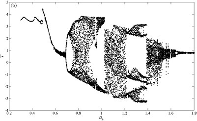
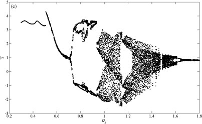
Fig. 6 presents four bifurcation diagrams for dimensionless dynamic transmission error of micro-segment gear system using dimensionless mesh frequency ${\mathrm{\Omega }}_k$ as bifurcation parameter. It can be observed that damping coefficient has a great effect on bifurcation behaviors of the gear system. The jump phenomena and chaotic area change much as damping coefficient increases.

Fig. 6Bifurcation diagrams using Ωk as bifurcation parameter: a) ζ= 0.06; b) ζ= 0.08; c) ζ= 0.1; d) ζ= 0.12

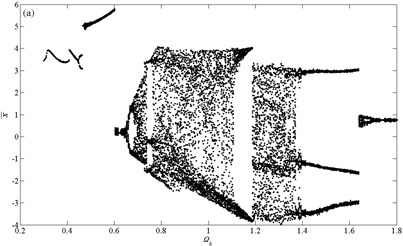
The bifurcation characteristic for the case of $\zeta =\mathrm{}$0.06 is shown in Fig. 6(a). It can be found that the motion is non-harmonic-single-periodic (NHS-periodic) at low values of dimensionless mesh frequency, i.e. ${\mathrm{\Omega }}_k\le \text{0.446}$. The response period $T$ of time history chart equals to excitation period, the phase diagram is a closed non-circle and non-elliptic curve, the resulting trace in Poincare map is a dot and the discrete points locate at the frequencies of $m{f}_k$ (where, $m$ is a positive integer, $f_k={\mathrm{\Omega }}_k/2\pi$, similarly hereinafter) in corresponding FFT Spectrogram according to Fig. 7(a). In the meantime, the first distinct amplitude jump happens at ${\mathrm{\Omega }}_k=\text{0.41}$.

Fig. 7Simulation results for some important values of Ωk when ζ=0.06: a) NHS-periodic at Ωk=0.25; b) 2T-periodic at Ωk=0.45; c) NHS-periodic at Ωk=0.552; d) 2T-periodic at Ωk=0.668; e) chaotic at Ωk=0.72; f) 3T-periodic at Ωk=0.752; g) 2T-periodic at Ωk=1.182; h) 3T-peiodic at Ωk=1.38; i) 2T-periodic at Ωk=1.67; j) simple harmonic at Ωk=1.74

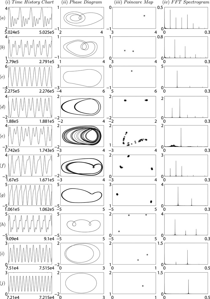
The motion mutates to be 2T-periodic as ${\mathrm{\Omega }}_k$ reaches 0.448 and this status continues to ${\mathrm{\Omega }}_k=\text{0.464}$, as shown in Fig. 7(b), the dominant peaks in FFT Spectrogram are $i{f}_k/2$, where, $i$ is an even number. The frequency $j{f}_k/2$, where $j$ is an odd number, lead to two deflected and closed cures in phase diagram. After the second jump at ${\mathrm{\Omega }}_k=\text{0.464}$, the system comes to be repeatedly transform between NHS-periodic and 2T-periodic motion until ${\mathrm{\Omega }}_k$ gets 0.492. The NHS-periodic motion lasts to ${\mathrm{\Omega }}_k=\text{0.66}$ and the third jump occurs at ${\mathrm{\Omega }}_k=\text{0.604}$.

As the dimensionless frequency ${\mathrm{\Omega }}_k$ further increases, the dynamic behavior of the system reverts to a 2T-periodic motion again at $\text{0.662}\le {\mathrm{\Omega }}_k\le \text{0.682}$. Here, two closed curves appear in the phase diagram and the dominant peaks in FFT Spectrogram are $m{f}_k/2$ which is different with the formal 2T-periodic motion.

After that, the motion evolves to be unstable, even chaotic in the range of $\text{0.684}\le {\mathrm{\Omega }}_k\le \text{0.738}$. When the dimensionless frequency ran up to 0.74, the system exhibits 3T-periodic motion, as shown in Fig. 7(f), the trajectories repeat themselves every three periods, and there are three discrete points on the Poincare map. The corresponding FFT spectrogram has peaks at the points of $m{f}_k/3$, but the situation just last for a while, the system turns back to be chaotic.

The state of chaos changes to be stabilized slowly, the system presents obvious 2T-periodic motion when ${\mathrm{\Omega }}_k$ reaches to 1.104, and its stability is getting better and better as ${\mathrm{\Omega }}_k$ increases until it comes to 1.186. The chaotic motions appear again in the range of $\text{1.186}\le {\mathrm{\Omega }}_k\le \text{1.37}$.

For dimensionless frequency $\text{1.372}\le {\mathrm{\Omega }}_k\le \text{1.638}$, the dynamic solutions are 3T-periodic. What’s more, the system experiences an impressive jump at next moment, and its solution turns to be 2T-periodic at $\text{1.668}\le {\mathrm{\Omega }}_k\le \text{1.696}$ after a brief struggle against unstable state ($\text{1.64}\le {\mathrm{\Omega }}_k\le \text{1.644}$ and $\text{1.652}\le {\mathrm{\Omega }}_k\le \text{1.666}$) and 2T-periodic state ($\text{1.646}\le {\mathrm{\Omega }}_k\le \text{1.65}$).

Finally, at high values of the dimensionless frequency, i.e. ${\mathrm{\Omega }}_k\ge \text{1.698}$, the dynamic behaviors keep simple harmonic, with an ellipse in phase diagram, one point in Poincare map and one frequency in FFT spectrogram, as show in Fig. 7(j).

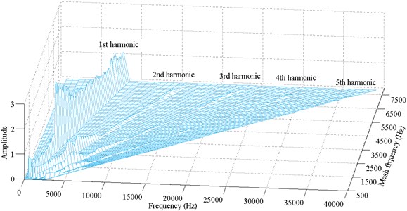
The frequency response amplitude for the system is shown in Fig. 8.

Fig. 8Frequency response amplitude at various mesh frequency for ζ=0.06

In the case of$\mathrm{}\zeta =\text{0.08}$, it can be seen that the maximum vibration amplitude decreases according to Fig. 6(b). The system performs NHS-periodic motion in the range of ${\mathrm{\Omega }}_k\le \text{0.472}$. An impressive jump happens at next moment, and the system presents 2T-periodic motion at the same time. Before long, the motion turns back to be NHS-periodic start from ${\mathrm{\Omega }}_k=\text{0.49}$, with the second jump. As ${\mathrm{\Omega }}_k$ increases to 0.6, the motion becomes unstable, and bifurcates into 2T-periodic motion at ${\mathrm{\Omega }}_k=\text{0.69}$ gradually.

As the dimensionless frequency further increases, the system comes into an unstable even chaotic state start from ${\mathrm{\Omega }}_k=\text{0.72}$, and then goes back to a stable 2T-periodic motion slowly at ${\mathrm{\Omega }}_k=\text{0.94}$. After a distinct jump at ${\mathrm{\Omega }}_k=\text{1.024}$ and a chaotic area $\text{1.026}\le {\mathrm{\Omega }}_k\le \text{1.214}$, the 2T-periodic motion evolves to be 3T-periodic. What’s more, the3T-periodic motion further evolves to be 6T-periodic at ${\mathrm{\Omega }}_k=\text{1.33}$.

With another jump happens at ${\mathrm{\Omega }}_k=\text{1.39}$, and in the following range of $\text{1.392}\le {\mathrm{\Omega }}_k\le \text{1.632}$, the system is mainly under chaotic or unstable state, besides the simple harmonic state happens in $\text{1.542}\le {\mathrm{\Omega }}_k\le \text{1.546}$ and $\text{1.594}\le {\mathrm{\Omega }}_k\le \text{1.6}$, and 2T-periodic state happens in $\text{1.616}\le {\mathrm{\Omega }}_k\le \text{1.62}$. Then, the system exhibits 2T-periodic motion again in the range of $\text{1.634}\le {\mathrm{\Omega }}_k\le \text{1.692}$. It can be said that the system goes to 2T-periodic motion after the variation between chaos state, simple harmonic state and 2T-periodic state.

After that, the system leads to the area of simple harmonic motion.

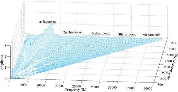
The diagram of frequency response amplitude for the system is shown in Fig. 9.

Fig. 9Frequency response amplitude at various mesh frequency for ζ=0.08

In Fig. 6(c), the system also exhibits NHS-periodic motion at low value of dimensionless frequency, i.e. ${\mathrm{\Omega }}_k\le \text{0.176}$, during this time, the first impressive jump appears at ${\mathrm{\Omega }}_k=\text{0.506}$. Then, the motion bifurcates to be 2T-periodic in the range of $\text{0.718}\le {\mathrm{\Omega }}_k\le \text{0.764}$, 4T-periodic in the range of $\text{0.766}\le {\mathrm{\Omega }}_k\le \text{0.858}$, 2T-periodic in the range of $\text{0.86}\le {\mathrm{\Omega }}_k\le \text{0.882}$ and 4T-periodic in the range of $\text{0.884}\le {\mathrm{\Omega }}_k\le \text{0.952}$. The second notable jump happens at ${\mathrm{\Omega }}_k=\text{0.938}$. After that, the system tends to be unstable even chaotic until ${\mathrm{\Omega }}_k$ gets 1.134. A 3T-periodic motion appears in the range of $\text{1.134}\le {\mathrm{\Omega }}_k\le \text{1.22}$. Subsequently, the dynamic solution goes to be chaotic again as ${\mathrm{\Omega }}_k$ rise from 1.222 to 1.472.

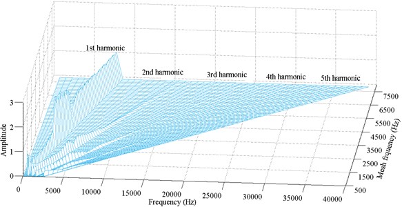
Fig. 10Frequency response amplitude at various mesh frequency for ζ=0.1

As the dimensionless frequency further increases, the system exhibits simple harmonic motion before the unstable motion presents again at ${\mathrm{\Omega }}_k=\text{1.488}$. Then a 2T-periodic motion replaces the unstable motion at $\text{1.582}\le {\mathrm{\Omega }}_k\le \text{1.648}$. Finally, for the dimensionless frequency $\text{1.65}\le {\mathrm{\Omega }}_k\le \text{3}$, the system performs simple harmonic motion.

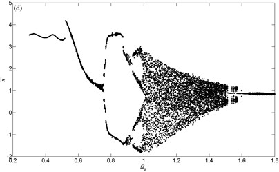
Fig. 6(d) reveals the bifurcation characteristics for $\zeta =\text{0.12}$ using dimensionless frequency ${\mathrm{\Omega }}_k$ as bifurcating parameter. Compared with the cases before, bifurcation characteristics here are much simpler. The system exhibits NHS-periodic motion in the range of ${\mathrm{\Omega }}_k\le \text{0.748}$, and then bifurcates to be 2T-periodic in the range of $\text{0.75}\le {\mathrm{\Omega }}_k\le \text{0.906}$. The motion further bifurcates to be 4T-periodic as ${\mathrm{\Omega }}_k$ increases to 0.908, and turn back to be 2T-periodic momently at $\text{0.918}\le {\mathrm{\Omega }}_k\le \text{0.93}$. Subsequently, the system goes to chaotic area start from ${\mathrm{\Omega }}_k=\text{0.99}$ after a 4T-periodic motion in the range of $\text{0.932}\le {\mathrm{\Omega }}_k\le \text{0.988}$.

Fig. 11Frequency response amplitude at various mesh frequency for ζ=0.12

The chaotic motion lasts for a long while until the simple harmonic motion replaces it at ${\mathrm{\Omega }}_k=\text{1.514}$. In the range of $\text{1.54}\le {\mathrm{\Omega }}_k\le \text{1.6}$, the motion shifts back and forth between 2T-periodic (sometime stable and sometime unstable) and simple harmonic. Finally, the response keeps simple harmonic at high values of ${\mathrm{\Omega }}_k$, i.e. ${\mathrm{\Omega }}_k\ge \text{1.602}$.

The bifurcation behaviors for the case of $\zeta =\text{0.04}$ and $\zeta =\text{0.14}$ are also investigated using the same method. The plots are not provided here in order to be brief. According to the bifurcation diagrams for different values of the dimensionless frequency, we can find that, impressive jump happens less time as damping coefficient increases.

The unstable and chaotic intervals are much affected as well. According to the discussion above, we can find that the intervals lead to unstable or chaotic responses have a trend to concentration as damping coefficient increases, as shown in Fig. 12.

Fig. 12Intervals of dimensionless frequency lead to unstable or chaotic solution

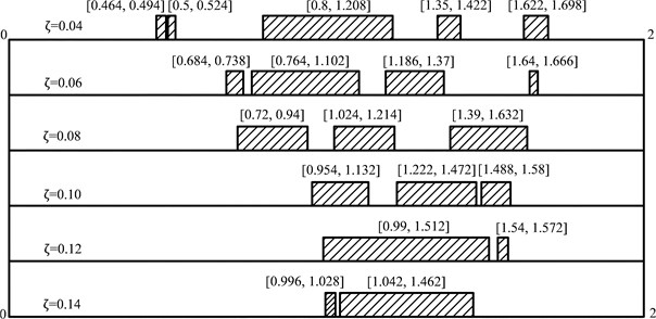
Moreover, the system is more sensitive to the dimensionless frequency at low value of damping coefficient, i.e., the type of motion changes more frequent as dimensionless frequency increases.

The rotational speed that probably causes an unstable or chaotic should be avoided to ensure stability and reliability of the system according to bifurcation diagrams.

3.2. Influence of external excitation

The fluctuation of torque is an important component of external excitation. To research the influence of fluctuation of torque on the bifurcation characteristics, both the fluctuation amplitude and the fluctuation frequency need significant consideration. Here, the system parameters are given as: ${\stackrel{-}{F}}_m=\text{0.05}$, $\xi =\text{0.25}$,${\overline{e}}_r=\text{0}$, ${\mathrm{\Omega }}_k=\text{0.2}$, $b=$20 μm.

Fig. 13 shows the bifurcation process of the system when ${\stackrel{-}{F}}_{p1}=\text{0.02}$, ${\mathrm{\Omega }}_p={\rho }_p{\mathrm{\Omega }}_k$, here ${\rho }_p$ is used as control parameter.

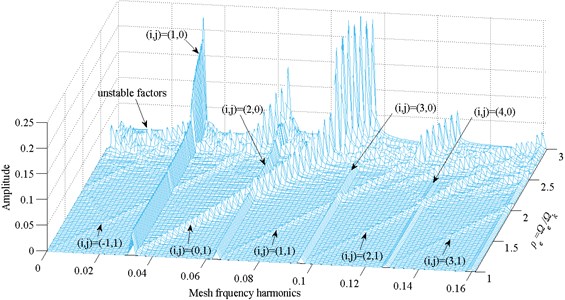
Fig. 13Bifurcation diagram using ρp as bifurcation parameter, here ρp=Ωp/Ωk

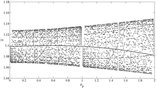
According to Fig. 15, the system presents an interesting bifurcation process. Two excitation sources result in a quasi-periodic motion with the response frequency $f_r=i{f}_k+j{f}_p$, here $f_k={\mathrm{\Omega }}_k/2\pi$, $f_p={\mathrm{\Omega }}_p/2\pi$, $i$, $j=$ 0, ±1, ±2,…. So, some special values of $\rho$ will lead to special motions

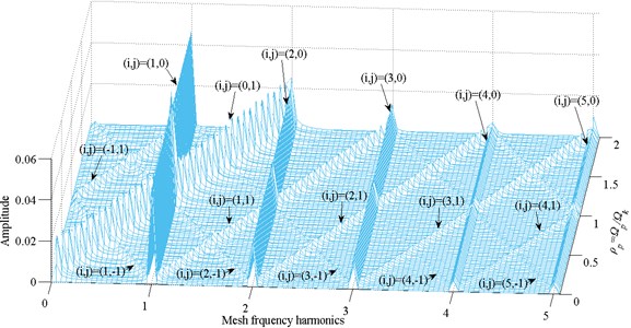
For example, in the case of ${\rho }_p=$0, 1, 2, the system exhibits NHS-periodic motion. In the case of ${\rho }_p=$0.5, 1.5, the system performs 2T-periodic motion. In the case of ${\rho }_p=$ 0.25, 0.75, 1.25, 1.75, the virbation response is 4T-periodic. In the case of ${\rho }_p=$0.2, 0.4, 0.6, 0.8, 1.2, 1.4, 1.6, 1.8, the system presents 5T-periodic motion. The corresponding frequency response amplitude diagram reveals the same situation, as shown in Fig. 14.

Fig. 14Frequency response amplitude at various external excitation frequency Ωp

Compared with the effect of external excitation frequency, the effect of external excitation amplitude is much simpler. The bifurcation diagram presented in Fig. 15 reveals that, at low values of ${\stackrel{-}{F}}_{p1}$, the system performs NHS- periodic motion. As ${\stackrel{-}{F}}_{p1}$ increases, the motion turns to be 4T-periodic due to the effect of external excitation frequency. What’s more, as ${\stackrel{-}{F}}_{p1}$ further increases, the motion keep 4T- periodic, the response amplitude is greatly affected.

The corresponding amplitude-frequency characteristic diagram presents the same situation, as shown in Fig. 16.

Fig. 15Bifurcation diagram using F-p1 as bifurcation parameter

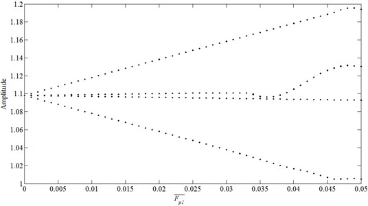
Fig. 16Frequency response amplitude at various external excitation amplitude F-p1

It can be found that, the response frequency is composed of non-dimensional frequency $f_k$ and external excitation frequency $f_p$; as ${\stackrel{-}{F}}_{p1}$ increases, the 4T-periodic motion is performed more obvious, and the amplitudes increase.

3.3. Influence of internal excitation

To investigate the influence of internal excitation on the bifurcation characteristics, the system parameters are assigned as follow: ${\stackrel{-}{F}}_m=\text{0.05}$, ${\stackrel{-}{F}}_{pr}=\text{0}$,$\xi =\text{0.25}$, ${\mathrm{\Omega }}_k=\text{0.2}$, ${\mathrm{\Omega }}_e={\rho }_e{\mathrm{\Omega }}_k$, ${\phi }_{er}=$ –0.72, $b=$20 μm. Here, both the influences of ${\mathrm{\Omega }}_e$ and ${\overline{e}}_r$ on bifucation characteristics are also investigated.

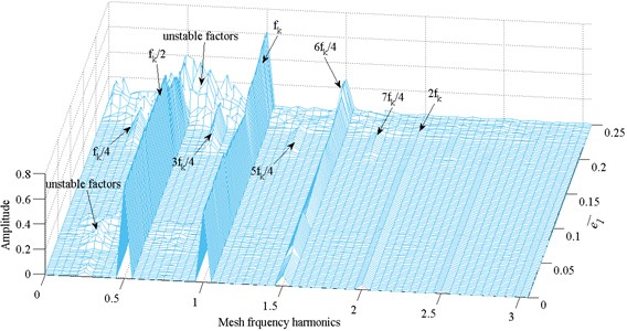
Fig. 17 shows the bifurcation characteristics of dimensionless dynamic transmission error by using ${\rho }_e$ as control parameter.

Similar to the bifurcation process using ${\rho }_p$ as bifurcation parameter, the response frequency of $\overline{x}$ also composed of the frequencies of two excitation sources, i.e. $f_r=i{f}_k+j{f}_e$. Here $f_k={\mathrm{\Omega }}_k/2\pi$, $f_e={\mathrm{\Omega }}_e/2\pi$, $i$, $j=$ 0, ±1, ±2,…. Similarly, special values of ${\rho }_e$ will lead to specail motions. In the case of, ${\rho }_e=$1, 2, 3, the system performs NHS-periodic motion. In the case of ${\rho }_e=$1.25, 1.75, 2.25, 2.75, the system exhibits 4-periodic motion. In the case of ${\rho }_e=$1.5, 2.5, the system presents 2T-periodic motion.

The difference is that, the response amplitude $\overline{x}$ has an obviously increase as ${\rho }_e$ increases, and when ${\rho }_e$ increases to 2.68, the system turns to be unstable. The corresponding amplitude-frequency characteristic diagram is shown in Fig. 18.

Fig. 17Bifurcation diagrams using ρe as bifurcation parameter, here e¯1=0.15

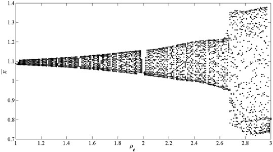
Fig. 18Frequency response amplitude at various internal excitation frequency Ωe

According to figure, it is clear that the response amplitude has a large jumping as ${\rho }_e$ increases, and the frequencies resulting in unstable motions are obviously increasing.

Fig. 19Bifurcation diagrams using e¯1 as bifurcation parameter, here Ωk=0.65

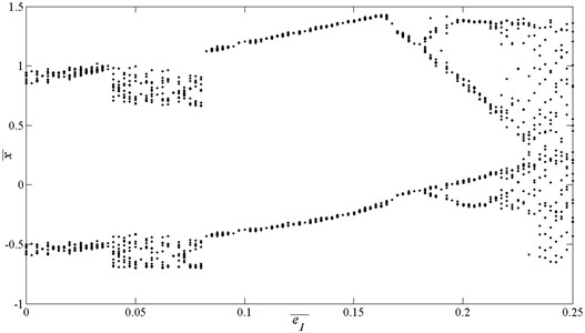
The bifurcation characteristics using ${\overline{e}}_1$ as control parameter is clearly presented based on Fig. 20. At the low values of ${\overline{e}}_1$, the system exhibits 2T-periodic motion. As ${\overline{e}}_1$ increases to 0.04, the motion becomes to be unstable. As ${\overline{e}}_1$ further increases to about 0.185, the motion bifurcates to be 4T-periodic. When ${\overline{e}}_1$ increases to 0.23, the system presents chaotic motion. According to the corresponding amplitude-frequency characteristic diagram, the unstable and chaotic phenomenon can be easily found. Another conclusion can be got, the growth of ${\overline{e}}_1$ has little influence on response amplitude, but has a great influence on the stability of the motion.

Fig. 20Frequency response amplitude at various internal excitation frequency e¯1

It can also be found that, the response frequency is composed of non-dimensional frequency $f_k$ and internal excitation frequency $f_e$; as ${\overline{e}}_1$ increases, the system bifurcates from 2T-periodic motion to 4T-periodic motion. The system performs chaotic motion as ${\rho }_e$ increases to 2.68 or as ${\overline{e}}_1$ increases to 0.23.