Improved algorithm of three-dimensional beamforming based on spatial cross-array

Song, Shaoyu; Xu, Zhongming; Li, Shu; Chen, Si; Zhang, Zhifei; He, Yansong

doi:10.21595/jve.2016.17006

Journal of Vibroengineering

Browse Journal

Submit article

Published: 31 December 2016

Check for updates

Improved algorithm of three-dimensional beamforming based on spatial cross-array

Shaoyu Song¹

Zhongming Xu²

Shu Li³

Si Chen⁴

Zhifei Zhang⁵

Yansong He⁶

^{1, 2, 3, 4, 5, 6}State Key Laboratory of Mechanical Transmission, Chongqing University, Chongqing 400044, China

^{1, 2, 3, 4, 5, 6}School of Automotive Engineering, Chongqing University, Chongqing 400044, China

Corresponding Author:

Zhongming Xu

Cite the article Download PDF

Downloads 1813

Abstract

Three-dimensional beamforming based on microphone array signal processing is the expansion of traditional 2D beamforming. However, its identification accuracy is often badly reduced by the effect of grating lobes and side lobes. To overcome this problem, a method called the hybrid method beamforming (HMB) combining functional generalized inverse beamforming with multiplicative filter of spatial cross-array is proposed. In this method, the statistically optimal processing and iterated generalized inverse beamforming with regularized matrix function are utilized to obtain initial result. Then the high order function is applied to filter the output. Subsequently, a novel non-uniform spatial cross-array optimized by genetic algorithm is used to obtain sound pressure distribution. The array consists of three orthogonal sub-arrays. Mutual cancellation is realized by computing respectively with data of sub-arrays and multiplying together. With fewer microphones, the result of the improved method can be obtained with a higher spatial resolution. The proposed method is verified by the simulation and the source localization test in a room. Compared with the conventional frequency domain beamforming (FDBF) algorithm and statistically optimal array processing (SOAP) beamforming, the performance of the proposed method is significantly improved in terms of resolution of the acoustic source.

1. Introduction

Beamforming is an important method based on array signal processing for noise source identification [1]. For the convenience of sensors arrangement and efficiency in the relatively poor test environment, beamforming is getting more and more widespread attention [2, 3]. In the conventional beamforming method, a scanning plane is dispersed into points first. Then the sound pressure at each point is computed using certain beamforming algorithm. By comparing the values of focal points, the source location is identified. To improve the resolution of beamforming, several algorithms, such as statistically optimal array processing (SOAP) [4, 5] adaptive beamforming [6, 7] and generalized inverse beamforming (GIB) [8, 9] were developed in the last decade. Unfortunately, they are restricted to the condition of known distance when they scan the plane. If the sources are not in the same plane, it may lead to large errors. Therefore, to overcome the shortcomings of unknown depth information, the 3D beamforming that extends scanning points to 3D space is developed.

To improve the spatial resolution of 3D beamforming, the common methods used are traditional frequency domain beamforming (FDBF) combined with deconvolution techniques. Ennes [10] found that FDBF without deconvolution became invalid when two-dimensional beamforming was extended to three-dimensional beamforming. Additionally, Ennes compared different spatial filter characteristics of four steering vectors in the field of 3D beamforming [11]. Brooks et al. [12] successfully applied 3D-DAMAS method to deconvolve the noise source map; Mathew [13] found that 3D CLEAN-SC has better resolution on the conditions of high-frequency and near-field after comparing deconvolution techniques of 2D CLEAN-SC and 3D CLEAN-SC. However, the faults of deconvolution techniques, which remove side lobes through iteration, are distinct. Large amount of calculation is required, and low efficiency is caused by massive focal points. Furthermore, other shortcomings, for example hypothesis of array pattern comes entirely from point spread function (PSF), remains to be improved.

As to the array geometry, the planar array has better spatial resolution in lateral direction than depth direction. The resolution will be poor if the scanning plane is placed normal to the array. It is usually not feasible to perform 3D beamforming with plane array [14, 15]. Therefore, Padois et al. [16] obtained relatively good results utilizing four spiral arrays surround sound source in the wind tunnel. However, its application is obviously limited by the needs of huge number of sensors. After simplifying the array geometry, Ric Porteous [17] proposed arrangement of two orthogonal planar spiral arrays. Four kinds of three-dimensional beamformers were compared. Consequently, the number of sensors is reduced.

The present paper aims at improving the location identification accuracy of 3D beamforming using fewer sensors. To achieve this goal, a hybrid method beamforming (HMB) and novel spatial cross-array are developed. The main idea of HMB is to reformulate the acoustic inverse problem combining SOAP and GIB with functional beamforming (FB) [18]. First, the priori information of sources defined by infinite norm is introduced into iterated SOAP processing which employs GIB algorithm. Second, the previous result is transformed into cross spectral matrix (CSM). High solution output with less side lobes is obtained after the processing of high order function. Subsequently, to reduce the number of sensors and make full use of the high resolution in the lateral direction, a optimal spatial cross-array is proposed by Genetic Algorithm.

The arrangement of rest parts are as follows: the hybrid method beamforming is introduced in Section 2.1. The form of spatial cross-array and principle of multiply filter are described in Section 2.2. Optimization using genetic algorithm is present in Section 2.3. In Section 3, the numerical simulation of proposed methods and comparisons with FDBF and SOAP of single and double sound sources are carried out. Section 4 provides some actual experimental results performed in a room.

2. Improved algorithm of the three-dimensional beamforming

2.1. Principle of the hybrid method beamforming

First, to suppress side lobes and improve the spatial resolution of 3D beamforming, the hybrid method beamforming is introduced. The priori information of sources and functional process are used to filter the result of SOAP beamformer. Consider an array of $M$ microphones whose coordinates are $x_{i} = (x_{i}, y_{i}, z_{i})$ . The number of focus points in 3D space is $N$ . The coordinate of acoustic source is $x_{t} = (x_{t}, y_{t}, z_{t})$ . The sound pressure of microphones is given by Eq. (1):

1

p (x_{i}) = G (x_{i}, x_{t}) q (x_{t}),

where $G$ is the free-field Green function between themicrophones and the sources. The elements of $G$ are $g_{i t} = e^{- j k R_{i t}} / R_{i t}$ and $q (x_{t})$ denotes the amplitude of sound source strength. To resolve the minimization problem, the problem described in Eq. (1) can be reformulated as:

2

m i n \{{‖p - G q‖}_{2}^{2} + β {‖L q‖}_{2}^{2}\},

where $β$ is a regularization parameter. $L$ is a regularization matrix used to regularize the solution. In general, we can obtain the result of Eq. (2) by getting the derivative of cost function in Eq. (2) to 0. While we can also solve it iteratively with statistically method. The solution is:

3

q^{(n + 1)} = L^{(n + 1)} {\underline{G}}^{H} α p,

where $\underline{G} = [\underline{g_{1}}, \underline{g_{2}}, \dots, \underline{g_{N}}]$ that defined as $\underline{G} = G L^{(n)}$ , which is the Green function having been modified.The superscript $H$ denotes Hermitian transpose. The expression of $α$ is $α = (\underline{G} {\underline{G}}^{H} + β I)^{- 1}$ . $β$ is related to signal-to-noise ratio (SNR). Simulation results show that $β$ is reasonable to be 0.1-10 % of the maximum eigenvalue of $\underline{G} {\underline{G}}^{H}$ . Finally, the normalized pressure of $t$ th focus point is written as:

4

Q_{t} = \frac{\underline{g_{t}^{H}} α p}{\underline{g_{t}^{H}} α g_{t}} = w_{t} p,

where the dimension of $w_{t}$ is [ $M$ , 1]. Taking all the scanning point together, Eq. (4) can be rewritten as:

5

Q = W p .

Here, the dimensions are $Q = [N, 1]$ , $W = [N, M]$ , $p = [M, 1]$ . Regularization matrix $L$ is defined as:

6

L = d i a g (\frac{|Q|}{{‖Q‖}_{\infty}}),

where $|.|$ means taking absolute value and ${‖.‖}_{\infty}$ denotes infinite norm and $d i a g (.)$ is rewriting vector into form of diagonal matrix. $L$ is an unit matrix in the first iteration and it is iteratively updated. Obviously, the elements of $L$ are limited between 0 and 1. The upper limit appears in the pack value of $Q$ . Blind regularization to the results is avoided in this way.

To improve the dynamic range of identification and suppress the side lobes furthermore, Eq. (6) is rewritten as the form of cross spectral matrix (CSM):

7

Q_{B F} = Q Q^{H} = W C W^{H} .

In Eq. (7), $Q_{B F}$ is the output and $C$ is cross spectrum matrix. The $C$ can be spectral decomposed as follows:

8

C = U Σ U^{'},

where $U$ is sa unitary matrix which consists of the eigenvectors of matrix $C$ . $U$ is the function of scanning points position. The middle term $Σ$ is a diagonal matrix which consists of corresponding eigenvalue of $C$ . Then we can define a high order matrix function as follows:

9

f^{(v)} (C) = U f^{(v)} (C) U^{'} = U d i a g [f^{(v)} (σ_{1}), \dots, f^{(v)} (σ_{N})] U^{'},

where $f^{(v)}$ is defined to be $f^{(v)} = t^{1 / v}$ . According to the theory of functional beamforming, outputs of functional beam former is:

10

Q_{F} = {(W C^{1 / v} W^{H})}^{v} .

Eq. (10) will degenerate into FDBF if $v = 1$ . Side lobes can be suppressed and dynamic range will be improved when $v$ is chosen to be larger than 1. Theoretically, the PSF outside the grating lobes and main lobe will exponentially decrease.

2.2. Multiplicative 3D beamforming based on spatial cross-array

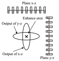
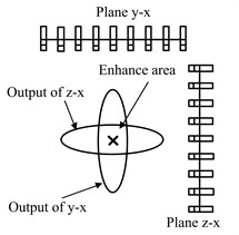
To reduce the number of sensors, the multiplicative 3D beamforming is proposed based on spatial cross-array. The spatial cross-array consists of three plane sub-arrays (illustrated in Fig. 1). Each sub-array has better resolution in the lateral direction. Spatial filtering is achieved after computing respectively and multiplying together. Therefore, complex computation of 3D deconvolution is averted.

Fig. 1Illustration of multiplicative 3D beamforming

Considering an array with 27 sensors consists of three sub-arrays. Each sub-array has 9 microphones. The sub-arrays are denoted as $S_{1}$ , $S_{2}$ and $S_{3}$ , respectively. The spatial relative locations are shown in Fig. 2. Each sensor is used twice, this leads to 54 receivers in the calculation. We structure three diagonal coefficient matrices $X_{1}$ , $X_{2}$ and $X_{3}$ sized 54×54. The definition is as follow:

11

X_{i i} = \{\begin{matrix} 1, & i \notin sub-array, \\ 0, & other . \end{matrix}

Fig. 2Structure of spatial cross-array to be optimized

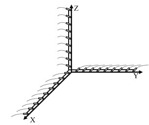
a) Three axes

b) One axis

The outputs of each sub-array are individually obtained with HMB. The results are as follows:

12

Q_{F 1} = {(W X_{1} C^{1 / v} X_{1} W^{H})}^{v},

13

Q_{F 2} = {(W X_{2} C^{1 / v} X_{2} W^{H})}^{v},

14

Q_{F 3} = {(W X_{3} C^{1 / v} X_{3} W^{H})}^{v} .

Then, Eqs. (12-14) are multiplied together and the cubic root is extracted as:

15

Q_{F i n a l} = \sqrt[3]{Q_{F 1} Q_{F 2} Q_{F 3}} .

Notably, Eq. (15) can only be utilized to the source localization. For one thing, the normalization is employed in the earlier processing; for another, functional beamformer’s output is always smaller than the true value. The source strength can be estimated with other methods.

2.3. Optimization of spatial cross-array based on genetic algorithm

Random geometry provides various spatial sampling intervals and thereby suppress the spatial aliasing problems. Unfortunately, to get these sampling intervals, the relatively large number of microphones is required. At the same time, the tedious trial and error cycle are often essential when design random geometries. For large random array, for example 1 m×1 m×1 m in this paper, it is difficult to build support structure and the cabling. Accordingly, the optimization algorithm is employed to get nonuniform and suitable array. Taking the symmetry of the sparse array [19, 20] into consideration, it is reasonable to search the optimal solution in one axis then expand the solution into three axes. The amount of calculation can be reduced in this way. To describe the ability of identifying the location of sound source, output in the adjacent area is regarded as side lobe. Schematic diagram is illustrated in Fig. 2. Then the main lobe energy level function $L$ is defined as follow:

16

L = l g (\frac{\int_{S_{0}}^{} {|p_{F}|}^{2} d s}{\int_{S}^{} {|p_{F}|}^{2} d s}),

In Eq. (16), $S_{0}$ is a small area contains the sound source, $S$ is the entire scan area. Optimization target can be expressed as: by setting the position of array element to maximize the sound source, namely $L$ , writen as:

17

\min \{- L (p_{F} (∆_{1}, ∆_{2}, \dots, ∆_{9}))\},

s . t . \{\begin{matrix} ∆_{i} \in (0,1), i = 1, 2, \dots, 9, \\ \min (∆_{i + 1} - ∆_{i}) \geq 0.03125, \end{matrix}

where $∆_{i}$ ( $i =$ 1,…, 9) is the value of microphone coordinate, and $p_{F}$ is the function of elemental position $∆_{i}$ . Adding minus sign to the right hand of Eq. (16). The objective function of Eq. (17) is nonnegative defined. The coordinate of each axis is between 0 and 1 meter. Moreover, to meet the restrict of minimum microphone distance, the bit of binary encoding is set to 5. Namely, the minimum spacing $m i n (∆_{i + 1} - ∆_{i})$ is ${(1 / 2)}^{5} =$ 0.03125 m. Nonuniform design usually leads to complex nonlinearities [21]. The deterministic optimization easily plunges into the local optimum. Evolutionary algorithms are taken into consideration. Note that the problem may not be continuously differentiable, so Genetic Algorithm is applicable to the issue. Other parameters are set as follows: number of individuals is 20, crossover rate is 0.7, mutation rate is 0.07, and the termination generation is 100. The optimized results are shown in Table 1. The convergence results of optimization are indicated in Fig. 3. Obviously, when the generation approaches 70, the optimization effect nearly reach the global optimum. The target function can be minimized with the elemental distribution in which the minimum spacing is 0.032 meter.

Table 1Optimal elements coordinates in one axle

Element number $i$	1	2	3	4	5	6	7	8	9
Coordinate	0.129	0.193	0.258	0.483	0.645	0.677	0.709	0.838	0.935

Ultimately, optimal element position in three axes are obtained after mirrored expanding of the solution space. The optimized results of spatial cross-array are shown in Table 2. The array is rotational symmetry in three axes.

Fig. 3The convergence results of genetic algorithm

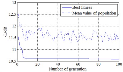
Table 2Optimal element coordinates in three axes

Element number $i$	1	2	3	4	5	6	7	8	9
Coordinate $x$	0.12	0.19	0.25	0.48	0.64	0.67	0.70	0.83	0.93
Element number $i$	10	11	12	13	14	15	16	17	18
Coordinate $y$	0.12	0.19	0.25	0.48	0.64	0.67	0.70	0.83	0.93
Element number $i$	19	20	21	22	23	24	25	26	27
Coordinate $z$	0.12	0.19	0.25	0.48	0.64	0.67	0.70	0.83	0.93

3. Verification of 3D beamforming using synthetic data

To demonstrate the performance of the proposed method, several examples of 3D sources identification utilizing synthetic data are provided with the proposed method based on spatial cross-array with 27 sensors designed in Section 2. In these cases, the set-up is as shown in Fig. 4. In all these calculations, 3D scanning area contained 226981 points in a cube measuring 0.6 m×0.6 m×0.6 m. The spacing of grid was chosen to be 0.01 m. The scope of the three coordinates was 0.2 m-0.8 m. The FDBF, and SOAP proposed by ref. [5] and HMB proposed in this work were compared. The regularization parameters $β$ of SOAP algorithm and HMB were selected to be 1 % of the maximum eigenvalue of $\underline{G} {\underline{G}}^{H}$ which is related to SNR. For convenience, all the results were normalized to display in the sound pressure distribution maps.

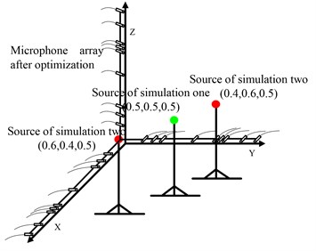
Fig. 4The set-up of simulation. The red solid circles are sources located at (0.4, 0.6, 0.5) m and (0.6, 0.4, 0.5) m, and the green solid circles is source located at (0.5, 0.5, 0.5) m

The set-up of simulation. The red solid circles are sources located at (0.4, 0.6, 0.5) m and (0.6, 0.4, 0.5) m, and the green solid circles is source located at (0.5, 0.5, 0.5) m

3.1. Monopole source

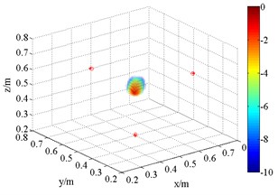
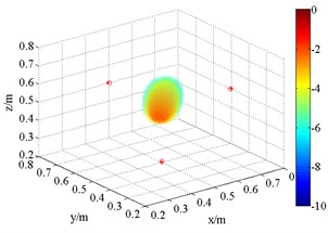
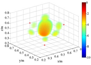
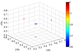
In the first simulation, a monopole source was located at (0.5, 0.5, 0.5) m. The set-up is as shown in Fig. 4. To approach actual impact, 15 dB Gauss white noise was added as background noise. In general, beamforming is used at medium and high-frequencies, so the frequency of acoustic source was set to be 3 kHz. The source maps obtained by different algorithms are shown in Fig. 5. To facilitate the observation, filter processing which filter the side lobes below –5 dB is actualized in Fig. 5. Contrastively, there is no such processing in Fig. 6.

Fig. 53D source maps of single monopole source. The symbols ‘○’ denote the projective position of the maximum outputs, and ‘*’ is that of theoretical

a) FDBF (3 kHz)

b) SOAP (3 kHz)

c) FDBF (1.5 kHz)

d) SOAP (1.5 kHz)

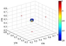
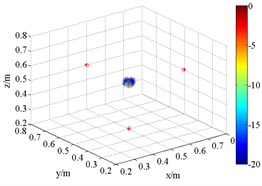
Fig. 63D source maps of single monopole source with HMB beamformer. The symbols ‘○’ denote the projective position of the maximum outputs, and ‘*’ is that of theoretical

3D source maps of single monopole source with HMB beamformer. The symbols ‘○’ denote the projective position of the maximum outputs, and ‘*’ is that of theoretical

a) HMB (1.5 kHz, $v =$ 1)

b) HMB (1.5 kHz, $v =$ 2)

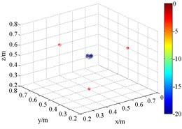
c) HMB (1.5 kHz, $v =$ 4)

d) HMB (3 kHz, $v =$ 1)

e) HMB (3 kHz, $v =$ 2)

f) HMB (3 kHz, $v =$ 4)

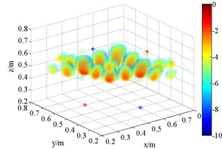
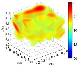
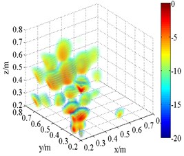
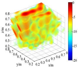
As shown in Fig. 5, FDBF and SOAP beamformer can identify the approximate location of the sound source at the frequency of 3 kHz. However, like others [22], it finds that they suffer a lot from side lobes, and the localization accuracy decreases with reduction of frequency. At the frequency of 1.5 kHz, the main lobes are merged with side lobes, making these two methods invalid although the theoretical point locates near the acoustic center. Meanwhile, at high frequency, the appearance of grating lobes in the sound pressure distribution with SOAP makes this method worse than FDBF algorithm.

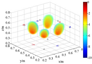
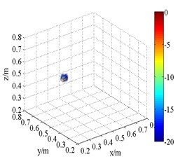
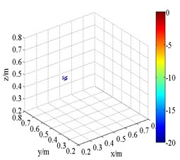
As shown in Fig. 6, the source maps with different frequency are obtained with different order $v$ in HMB beamformer. In the program, the number of iterations is 4. The dynamic range of display is set between 0 and –20 dB. Obviously, the position of the maximum pressure appears extremely near the theoretical location, namely (0.5, 0.5, 0.5) m. Compared with the outputs of FDBF and SOAP beamformer (Fig. 5), the width of main lobe in the source maps is successfully decreased. The accuracy of sound source identification is greatly improved.

Meanwhile, it is clear that the resolution is related to order. In theory, the functional beamforming will reduce to FDBF for $v =$ 1. Therefore, Fig. 6(a) and (d) are also the computing results of formula replacing $Q_{F}$ in Eq. (15) with $Q_{B F}$ in Eq. (7). With the increases of order $v$ , such as $v =$ 2 and 4, the main lobe of the outputs of HMB algorithm turns sharper. The position of acoustic source is well identified. The reason for Fig. 6(a) and (d) have better resolution compared with (a), (b) and (c), (d) in Fig. 5 respectively is that HMB introduces regularization matrix $L$ which takes the location of sound source into account to iteratively filter and results. For ill condition problem, it is an effective idea.

3.2. Coherent sources

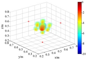
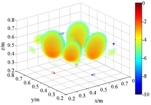
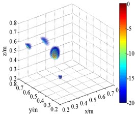
In the second simulation, two coherent acoustic sources were located at (0.6, 0.4, 0.5) m and (0.4, 0.6, 0.5) m respectively. Other conditions, such as background noise and frequency, were the same as values in application one. Similarly, FDBF and SOAP beamforming algorithms were employed to recover the sound pressure produced by sources in 3D space. The results (Fig. 7) show that grating lobes symmetrically appear beside actual sources at frequency of both 1.5 kHz and 3 kHz. In this case, the strength of main lobes and grating lobes are approximate. Neither of them locates the two coherent sources well. This phenomenon is actually caused by space sampling. This finding demonstrates that the anti-aliasing capability of FDBF and SOAP is poor. More grating lobes appear at the frequency of 3 kHz compared with that of 1.5 kHz. On the one hand, the source frequency must be low to avoid this effect; on the other hand, the resolution of low frequency is inferior. It limits the application of 3D beamforming.

Fig. 73D source maps of coherent acoustic sources with FDBF and SOAP. The symbols ‘○’ denote the projective position of the maximum outputs, and ‘*’ is that of theoretical

3D source maps of coherent acoustic sources with FDBF and SOAP. The symbols ‘○’ denote the projective position of the maximum outputs, and ‘*’ is that of theoretical

a) FDBF (3 kHz)

b) SOAP (3 kHz)

c) FDBF (1.5 kHz)

d) SOAP (1.5 kHz)

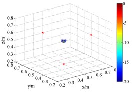
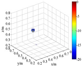
Fig. 8 is the output of sound pressure with HMB algorithm. It shows that HMB is able to localize the coherent acoustic sources in 3D space. With the same processing in the application one, the order $v$ is set to be $v =$ 1, 2 and 4 at each frequency respectively. The resolution of sources localization and its relationship with order $v$ are similar to the results in Fig. 6. Compared with FDBF and SOAP, the identification radius of HMB with a large order is remarkably decreased. Meanwhile, the sources are restricted within a relatively smaller 3D space. It verifies the coherent acoustic sources localization capability of proposed method from the perspective of simulation.

Fig. 83D source maps of emulational coherent acoustic sources. The symbols ‘○’ denote the projective position of the maximum outputs, and ‘*’ is that of theoretical

3D source maps of emulational coherent acoustic sources. The symbols ‘○’ denote the projective position of the maximum outputs, and ‘*’ is that of theoretical

a) HMB (1.5 kHz, $v =$ 1)

b) HMB (1.5 kHz, $v =$ 2)

c) HMB (1.5 kHz, $v =$ 4)

d) HMB (3 kHz, $v =$ 1)

e) HMB (3 kHz, $v =$ 2)

f) HMB (3 kHz, $v =$ 4)

4. Verification of performance using experimental data

To verify the validity and reliability of proposed method, an acoustic radiation model of single source was experimentally investigated in a room. It included one loudspeaker (D&S type 139-5) fixed in 3D scanning space. The radius of the loudspeaker membrane is 0.03 m. Loudspeakers are frequently used to model sound generating for its’ accessibility and reliability.

Fig. 9Hardware layout of incoherent sources and the virtual array

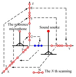
a) The hardware arrangement

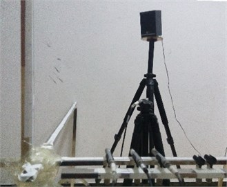
b) The experiment site

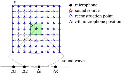
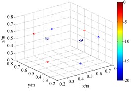
The hardware layout of experiment is shown in Fig. 9. The microphone array optimized in Section 2 was utilized. The array had 27 elements. To reduce the number of microphones, the scanning measurement method was used based on virtual array approach [23, 24]. In this way, three microphones (B&K Type 8192-A) were employed to collect the sound pressures at target locations. The pressures phase could be obtained by a fixed reference microphone (B&K Type 8192-A). The scan order of the three elements is shown in Fig. 9. Ultimately, the pressure data measured by 27 array elements can be obtained after 9 measurements.

In this experiment, the loudspeaker generated Gauss white-noise that was stationary in time-domain. Each of the sensors (four B&K Type 8192-A) was connected to a B&K data acquisition system with LAN-XI collector module. The sound data were acquired at a sampling frequency of 12.56 kHz, and the sampling time was 5 s. Before being processed by the algorithm, the measured pressure signals were firstly calculated by fast Fourier transform. The focusing grid and other parameters, like iterations and regularization parameter, were samely chosen as those in simulations.

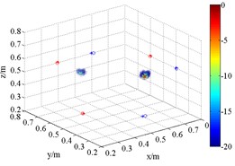
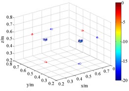
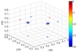
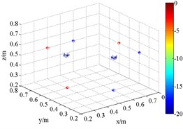
Fig. 10Experimental 3D beamforming source maps

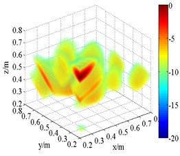
a) FDFB (1.5 kHz)

b) SOAP (1.5 kHz)

c) HMB (1.5 kHz, $v = 1$ )

d) HMB (1.5 kHz, $v = 4$ )

e) FDFB (2.5 kHz)

f) SOAP (2.5 kHz)

g) HMB (2.5 kHz, $v = 1$ )

h) HMB (2.5 kHz, $v = 4$ )

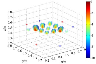
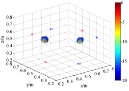
The 3D source maps calculated with data collected previously are shown in Fig. 10. The frequencies are presented in 1/3th octave bands via calculating integrating operation. The limits of integration correspond to lower and upper limits of frequency. In this way, the data of frequency centered at 1.5 kHz and 2.5 kHz are selected as input. The source position is detected via normalized values in source maps. As shown in Fig. 10, both FDFB and SOAP beamformer produce broad side lobes in the 3D space. The results are qualitatively similar to those of simulation. A number of fake sources appear in the scanning space. The main lobe position of speaker is merged with side lobes. Fig. 10(b) and (f) has larger beamwidths than Fig. 10(a) and (e) respectively. Compared with FDFB, SOAP fail to separate the main lobe. It shows the poor capacity of SOAP in the field of 3D beamforming. Additionally, Fig. 10(e) and (f) has narrower main lobe than Fig. 10(a) and (b) respectively because of the increase of frequency. That is a well-known character of beamforming. Unlike Fig. 10(a), (b) and (e), (f), the results of HMB beamformer (Fig. 10(c), (d), (g) and (h)) are of high quality. HMB algorithm yields much narrower main lobe. The resolution of 3D beamforming is improved thanks to the capability of the side lobes suppression of HMB. It is achieved by introducing iteration, which makes use of previous source distribution, and high order functional processing. Meanwhile, the effect of order $v$ on the results is studied. The source maps show that the main lobe is narrower with larger order. Namely, HMB with larger value of order can improve the resolution of localization to a certain degree under the same conditions. The dynamic range is increased at the same time. Not surprising, point spread function of the array is less than 1 outside the peak value, and it will exponentially decrease with the increasing of order. It results in narrow down of main lobes.

5. Conclusions

A novel three-dimensional beamforming algorithm for spatial localization of acoustic source is proposed, called hybrid method beamforming. By introducing the regularization matrix related to source distribution into optimal estimating, the equation of beamformer is inversely solved utilizing the generalized inverse algorithm. The dynamic range of identification can be improved by rewriting the solution into form of CSM followed by employing the method of functional beamforming. Meanwhile, side lobes can be suppressed in this processing. To reduce the number of sensors and make full use of the high resolution in the lateral direction, an innovative spatial cross-array is proposed. Ultimately, the mutual cancellation is achieved by computing respectively and multiplying together. The proposed method successfully improved the resolution of 3D beamforming with less sensors compared with arrays of [16, 17].

Both simulations and experiments carried out in a normal room have validated the effectiveness and correctness of proposed method. No characters of the sources are previously assumed with the principle of proposed method. Compared with FDBF and SOAP beamformer, hybrid method beamforming can effectively suppress side lobes and improve the accuracy of sound source localization. Moreover, with the increase of order, the proposed method sharpens the peak value of sources. Taken together, this work provides a potential method of multipole-source-detection with reasonably selecting of order.

References

Hald J. Combined NAH and beamforming using the same microphone array. Sound and Vibration, Vol. 38, Issue 12, 2004, p. 18-27.

Search CrossRef
Allen C. S., Blake W. K., Dougherty R. P., Lynch Denis, Soderman P. T., Underbrink J. R., Mueller T. J. Aeroacoustic Measurements. Springer Science and Business Media, Berlin, 2013.

Search CrossRef
Sydow C. Broadband beamforming for a microphone array. Journal of the Acoustical Society of America, Vol. 96, Issue 2, 1994, p. 845-849.

Publisher
Mao Jin, Xu Zhongming, He Yansong, Zhang Zhifei, Li Shu The improved separation method of coherent sources with two measurement surfaces based on statistically optimized near-field acoustical holography. Journal of Vibroengineering, Vol. 17, 2014, p. 674-681.

Search CrossRef
Pascal J. C., Li J. F. Use of double layer beamforming antenna to identify and locate noise sources in cabins. 6th European Conference on Noise Control: Advanced Solutions for Noise Control, 2006.

Search CrossRef
Li J., Stoica P. Robust Adaptive Beamforming. John Wiley and Sons Inc., New Jersey, 2006.

Publisher
Lee C. C, Lee J. H. Robust adaptive array beamforming under steering vector errors. Antennas and Propagation, IEEE Transactions on Antennas and Propagation, Vol. 45, Issue 1, 1997, p. 168-175.

Publisher
Suzuki Takao L1 generalized inverse beam-forming algorithm resolving coherent/incoherent, distributed and multipole sources. Journal of Sound and Vibration, Vol. 330, Issue 24, 2011, p. 5835-5851.

Publisher
Padois T., Gauthier P. A., Berry A. Inverse problem with beamforming regularization matrix applied to sound source localization in closed wind-tunnel using microphone array. Journal of Sound and Vibration, Vol. 333, Issue 25, 2014, p. 6858-6868.

Publisher
Sarradj E. Three-dimensional acoustic source mapping. 4th Berlin Beamforming Conference, 2012.

Publisher
Sarradj E. Three-dimensional acoustic source mapping with different beamforming steering vector formulations. Advances in Acoustics and Vibration, Vol. 2012, 2012, p. 292695.

Search CrossRef
Brooks T. F., Humphreys W. M. Three-dimensional application of DAMAS methodology for aeroacoustic noise source definition. AIAA Paper, Vol. 2960, 2005.

Publisher
Legg M., Bradley S. Automatic 3D scanning surface generation for microphone array acoustic imaging. Applied Acoustics, Vol. 76, 2014, p. 230-237.

Publisher
Brooks T. F., Humphreys W. M. Flap-edge aeroacoustic measurements and predictions. Journal of Sound and Vibration, Vol. 261, Issue 1, 2003, p. 31-26.

Publisher
Geyer T., Sarradj E., Giesler J. Application of a beamforming technique to the measurement of airfoil leading edge noise. Advances in Acoustics and Vibration, Vol. 2012, 2012, p. 905461.

Publisher
Padois T., Robin O., Berry A. 3D Source localization in a closed wind-tunnel using microphone arrays. AIAA Paper, Vol. 2213, 2013.

Publisher
Porteous R., Prime Z., Doolan C. J., Moreau D. J., Valeau V. Three-dimensional beamforming of dipolar aeroacoustic sources. Journal of Sound and Vibration, Vol. 355, 2015, p. 117-134.

Publisher
Dougherty R. P. Functional beamforming. 5th Berlin Beamforming Conference, 2014.

Search CrossRef
Hebib S., Raveu N., Aubert H. Cantor spiral array for the design of thinned arrays. IEEE Antennas and Wireless Propagation Letters, Vol. 5, Issue 1, 2006, p. 104-106.

Publisher
Meijer C. A. Simulated annealing in the design of thinned arrays having low sidelobe levels. Proceedings of the South African Symposium on Communications and Signal Processing, 1998, p. 361-366.

Publisher
Li M., Wei L., Fu Q., Yang D. Ghost image suppression based on particle swarm optimization-MVDR in sound field reconstruction. Journal of Vibration and Acoustics, Vol. 137, Issue 3, 2015, p. 031007.

Publisher
Petri Jarske, Tapio Saramaki, Sanjit K. Mitra, Yrjo Neuvo On properties and design of nonuniformly spaced linear arrays. IEEE Transaction on Acoustics, Speech, and Signal Processing, Vol. 36, Issue 3, 1988, p. 372-380.

Publisher
Comesana D. F., Wind J., Holland K., Grosso A. Far field source localization using two transducers: a virtual array approach. 18th International Congress of Sound and Vibration, 2011.

Search CrossRef
Comesana D. F., Holland K., Wind J., Bree H. E. D. Adapting Beamforming Techniques for Virtual Sensor Arrays. 4th Berlin Beamforming Conference, 2012.

Search CrossRef

About this article

Received

23 March 2016

Accepted

18 August 2016

Published

31 December 2016

SUBJECTS

Acoustics, noise control and engineering applications

DOI

https://doi.org/10.21595/jve.2016.17006

Keywords

three-dimensional beamforming

multiplicative filter

generalized inverse beamforming

high order function

noise source identification

Acknowledgements

This work was supported by the Foundation and Advanced Research Project of Chongqing (Grant No. CSTC2015jcyjBX0075).

Author Contributions

Shaoyu Song conceived and designed the work. Meanwhile, he wrote the main part of the program as well as drafted and revised the manuscript. Zhongming Xu contributed materials and analysis tools as well as approved the final version. Shu Li designed the experiments and helped to write the program. Si Chen helped to write and revise the manuscript as well as perform the experiments. Zhifei Zhang helped to acquire the data and drafted the manuscript. Yansong He gave constructive advice to this work.

This is an open access article distributed under the Creative Commons Attribution License, which permits unrestricted use, distribution, and reproduction in any medium, provided the original work is properly cited.

Previous article in issue Previous

Research article

2023 02 09

An improved deconvolution beamforming algorithm for acoustic imaging of low signal-to-noise ratio sound sources in reverberant field

Wenyong Guo, Hantao Chen, Jing Xia, Xiaofeng Li, Chenghao Cao

Research article

2022 06 13

A deconvolution sound source identification method based on twice weak selection orthogonal matching pursuit

Weipeng Zhao, Jin Mao, Kai Liu

Research article

2022 05 15

An adaptive beamforming algorithm for sound source localisation via hybrid compressive sensing reconstruction

Wenyong Guo, Jianggui Han, Hantao Chen, Li Yu, Zhe Wu

Research article

2019 12 31

Source localization in reverberation environment based on improved equivalent sound source near-field acoustic holography algorithm

Hongyu Zhang, Wenyong Guo, Jianggui Han, Hantao Chen

S. Song, Z. Xu, S. Li, S. Chen, Z. Zhang, and Y. He, “Improved algorithm of three-dimensional beamforming based on spatial cross-array,” Journal of Vibroengineering, Vol. 18, No. 8, pp. 5619–5631, Dec. 2016, https://doi.org/10.21595/jve.2016.17006

Copy Extrica

Copied to clipboard!

TY  - JOUR
DO  - 10.21595/jve.2016.17006
UR  - https://doi.org/10.21595/jve.2016.17006
TI  - Improved algorithm of three-dimensional beamforming based on spatial cross-array
T2  - Journal of Vibroengineering
AU  - Xu, Zhongming
AU  - Song, Shaoyu
AU  - Li, Shu
AU  - Chen, Si
AU  - Zhang, Zhifei
AU  - He, Yansong
PY  - 2016
DA  - 2016/12/31
PB  - JVE International Ltd.
SP  - 5619-5631
IS  - 8
VL  - 18
SN  - 1392-8716
ER  - 

Copy Ris

Copied to clipboard!

@article{Xu_2016,
	doi = {10.21595/jve.2016.17006},
	url = {https://doi.org/10.21595/jve.2016.17006},
	year = 2016,
	month = {dec},
	publisher = {{JVE} International Ltd.},
	volume = {18},
	number = {8},
	pages = {5619--5631},
	author = {Zhongming Xu and Shaoyu Song and Shu Li and Si Chen and Zhifei Zhang and Yansong He},
	title = {Improved algorithm of three-dimensional beamforming based on spatial cross-array},
	journal = {Journal of Vibroengineering}
}

Copy Bibtex

Copied to clipboard!

[1]Z. Xu, S. Song, S. Li, S. Chen, Z. Zhang, and Y. He, “Improved algorithm of three-dimensional beamforming based on spatial cross-array,” Journal of Vibroengineering, vol. 18, no. 8, pp. 5619–5631, Dec. 2016, doi: 10.21595/jve.2016.17006.

Copy IEEE

Copied to clipboard!

Xu, Zhongming, Shaoyu Song, Shu Li, Si Chen, Zhifei Zhang, and Yansong He. “Improved Algorithm of Three-Dimensional Beamforming Based on Spatial Cross-Array.” Journal of Vibroengineering 18, no. 8 (December 31, 2016): 5619–31. https://doi.org/10.21595/jve.2016.17006.

Copy Chicago

Copied to clipboard!

Improved algorithm of three-dimensional beamforming based on spatial cross-array

Abstract

1. Introduction

2. Improved algorithm of the three-dimensional beamforming

2.1. Principle of the hybrid method beamforming

2.2. Multiplicative 3D beamforming based on spatial cross-array

2.3. Optimization of spatial cross-array based on genetic algorithm

3. Verification of 3D beamforming using synthetic data

3.1. Monopole source

3.2. Coherent sources

4. Verification of performance using experimental data

5. Conclusions

References

About this article

Related Articles