Abstract
The generalization of the classical Korteweg-de-Vries (KdV) solitary wave solution is presented in this paper. The amplitude and the propagation speed of generalized KdV solitary waves vary in time. Generating partial differential equations and conditions of existence of the generalized KdV solitary waves are derived using the inverse balancing method. Computational experiments illustrate the variety of new solitary solutions and their generating equations.
1. Introduction
Solitary solutions of nonlinear partial differential equations play a major part in mathematical physics [1]. While most commonly solitary waves maintain constant amplitude and propagation speed (because they are obtained via the traveling wave substitution recent developments include solitary solutions which have either a variable amplitude or propagation speed, or both. It is demonstrated in [2] that soliton’s amplitude and width can alter during the propagation in the model of (2+1)-dimensional coupled nonlinear Schrodinger equations in a graded-index waveguide. It is shown that the maximum amplitude of the solitary solution to the (1+1)D CQNLS equation in the self-focusing quintic case does depend on the propagation distance [3].
A number of oscillating solitons such as the dromion and solitoff have been shown to satisfy the nonlinear (2+1)-dimensional Broer-Kaup (BK) equations in [4]. The deformed soliton, breather and rogue wave solutions of the inhomogeneous nonlinear Hirota equation with linear inhomogeneous coefficients and higher-order dispersion are discussed in [5]. The variational approach is employed in [6] to construct three classes approximate azimuthally modulated vortex solitons for the (2+1)-dimensional nonlinear Schrodinger equation with transverse nonperiodic modulation. Higher-order Dirac solitons, which have amplitude profiles that repeat periodically over large propagation distances are investigated in [7].
Solitary solutions are often considered in the context of birefringent optical fibers. In [8], an analytic model is constructed to demonstrate polarized soliton oscillations in a lossy elliptically low birefringent optical fiber. A study on the propagation of optical solitons through birefringent fibers in the presence of spatio-temporal dispersion is presented in [9]. The Riccati equation and Jacobian elliptic equation methods are used to study the propagation of optical solitons in birefringent fibers with parabolic law nonlinearity [10]. Bright and dark 1-soliton solutions of systems modeling birefringent fibers are considered using several perturbation terms in [11]. The dynamics of soliton propagation through optical metamaterials can be found in [12].
There have also been reports of experimental evidence of solitary solutions with non-constant speed and amplitude. A discussion on the way spiralling elliptic solitons can be observed experimentally can be found in [13]. A study on soliton frequency shifts in few-cycle ultrashort laser pulses propagating through resonant media has recently been published in [14]; self-decelarating Airy-Bessel light bullets are is discussed in [15].
Recent exact solitary solution derivation techniques have demonstrated that the field is no longer limited to the classical soliton. The curved soliton solution to the damped externally excited KdV equation has been obtained in [16]; the embedded and annula soliton solutions to the (2+1)-dimensional Burgers equation have been discussed in [17].
The main objective of this article is to provide an analytical framework for the determination of the generating equations which possess generalized solitary solutions with non-constant amplitude and propagation speed. The inverse balancing method is used to identify classes of nonlinear partial differential equations that admit such solitary solutions. Conditions of existence for generalized solitary solutions are derived; computational experiments illustrate the variety of new solitary solutions and their generating equations.
2. Korteweg-de-Vries solitary waves
It is well-known that the Korteweg-de-Vries (KdV) equation:
which models one-dimensional shallow water waves with small amplitudes does admit the solitary-wave solution:
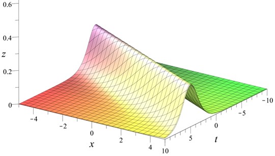
where , , are parameters that can be computed from Eq. (1) [1]. Note that corresponds to the constant propagation speed of the wave; corresponds to the amplitude and is the level of undisturbed water. The plot of Eq. (2) is given in Fig. 1.
In this paper, the following generalization of Eq. (2) is considered:
where corresponds to the variable amplitude of the solitary wave and to the propagation speed (which need not be constant). The functions , are continuous, differentiable and do not have essential singularities. This generalization allows the consideration of waves with soliton-like characteristics – but with variable speed and amplitude.
Fig. 1Classical KdV solitary wave Eq. (2) with α=s= 1
3. Generating equations of generalized KdV solitary waves
Partial differential equations that admit the solution Eq. (3) are derived in this section. Conditions of the existence of solutions Eq. (3) in a class of differential equations are considered.
3.1. Derivation of generating PDEs
Eq. (3) can be rewritten as:
Differentiating Eq. (4) with respect to , yields:
The inverse balancing can now be used: considering Eqs. (4), (5) algebraic equations, the variables and can be expressed as:
Inserting Eq. (6) into Eq. (4) yields the partial differential equation:
Returning to the original variables yields:
Thus Eq. (7) can be rewritten as:
Note that the generating equations of the classical KdV solitary solution Eq. (2) are special cases of Eqs. (7) and (9) when , 1, :
Both equations defined in Eq. (10) have solution Eq. (2). Subsequent differentiation and use of Eq. (10) yields the KdV Eq. (1).
The equations (9) are not integrable; however, it has been shown that solitary solutions exist in many nonintegrable systems [18]. Furthermore, their properties can be different than those that are encountered in integrable systems, including non-constant amplitude and propagation speed [18].
3.2. Derivation of generalized solitary solutions and their conditions
Suppose the following partial differential equation is given:
where , , are known functions of , . Comparing Eqs. (9) and (11) yields that Eq. (11) admits the generalized KdV solitary solution Eq. (3) if the following equations hold:
Eqs. (13), (14) yield:
Let us introduce the function :
Note that depends only on , because .
The consistency condition and Eqs. (12)-(14) results in the constraint:
Furthermore, if only real-valued solutions are considered, the condition:
must be satisfied. Then Eqs. (13), (14) have the solution:
From Eqs. (15) and (19) it follows that the parameters of the generalized KdV solitary wave read:
Note that:
for all , thus only the positive-sign branch of Eq. (21) is considered further in this paper.
3.3. Cauchy initial value problem on Eq. (11)
The Cauchy initial value problem on the partial differential Eq. (11) can be posed in the following way: given the Eq. (11), find a generalized KdV solitary solution Eq. (3) subject to initial conditions:
The derivations of Subsection 3.2 indicate the necessary and sufficient conditions for the solution to the discussed Cauchy problem. The partial differential Eq. (11) admits the generalized KdV solitary solution Eq. (3) if and only if the coefficients of the equation , , satisfy the conditions Eqs. (16), (17) and (18).
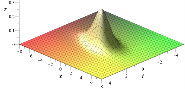
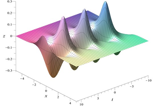
Fig. 2Decaying amplitude generalized KdV solitary wave Eq. (30) with t0= 0, u0= 1, x0=v0= 0
4. Several examples of generalized solitary solutions
4.1. Decaying amplitude solitary wave
Suppose the following partial differential equation is given:
The coefficients of the equation read:
Eq. (24) has a generalized KdV solitary solution because conditions Eqs. (16), (17) and (18) hold true. Eqs. (15) and (19) read:
The solution of Eqs. (26) and (27), according to Eqs. (20) and (21) reads:
Thus, the equation has the generalized solitary solution:
Note that the constants , only determine the location of the peak amplitude of the solitary wave. The plot of Eq. (30) is given in Fig. 2. The propagation speed of the solitary wave remains constant throughout all values of – but while the amplitude of the solitary solution decays in time.
4.2. Decaying amplitude solitary wave with variable speed
Suppose the following partial differential equation is given:
Eq. (31) together with Eqs. (15) and (19) yields:
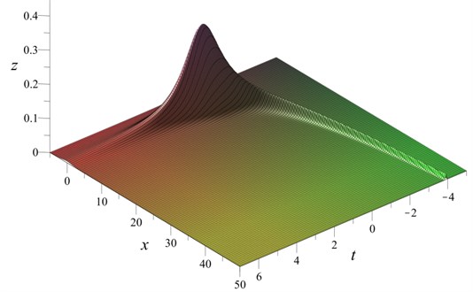
Fig. 3Generalized KdV solitary wave with decaying amplitude and variable speed Eq. (36) with t0= 0, u0= 1/10, x0= 0, v0= 1
According to Eqs. (20) and (21) integration results in the functions:
that yield the generalized solitary solution:
The plot of Eq. (36) is given in Fig. 3. Note that this solitary solution has decaying amplitude and a variable propagation speed.
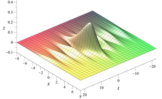
4.3. Solitary wave with bounded growing amplitude
Let the following partial differential equation be given:
Following the same steps as in the previous examples, it is obtained that:
Integrating yields the functions:
The solitary wave reads:
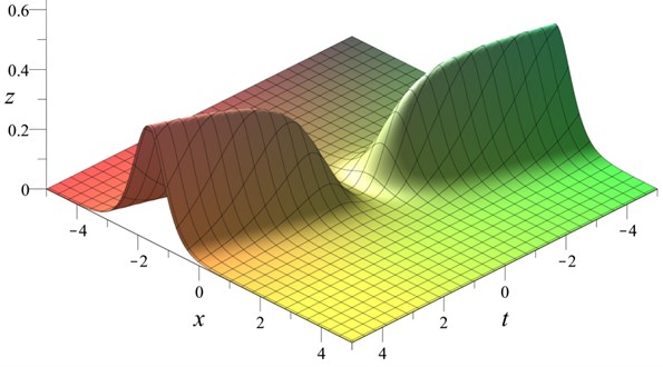
This type of generalized solitary solution has a growing amplitude as increases (or decreases) from (Fig. 4). However, the amplitude of the solitary wave does not increase unboundedly.
Fig. 4Generalized KdV solitary wave with bounded and growing amplitude Eq. (42) with t0=x0=u0=v0= 0
4.4. Breathers
4.4.1. Breather with constant amplitude
Suppose the following partial differential equation is given:
In this case, Eqs. (15) and (19) read:
Integrating Eqs. (44) and (45) yields the solitary solution:
Nonlinear waves such as Eq. (46), in which energy concentrates in an oscillatory fashion are called breathers [1]. The solution Eq. (46) is an example of a breather with constant amplitude: the amplitude of the wave varies for different , but it does not decay (Fig. 5).
Fig. 5Standing breather Eq. (46) with t0= 0, x0=u0= 1, v0= 2
4.4.2. Breather with decaying amplitude
Let the following partial differential equation be given:
Eqs. (15) and (19) read:
Integration of Eqs. (48) and (49) results in the solitary solution:
The obtained solution Eq. (50) is a type of breather which has decaying amplitude (Fig. 6).
5. Conclusions
It is shown that the classical Korteweg-de-Vries solitary wave can be generalized to represent solitary wave structures with variable amplitude and propagation speed. The generating equations that have generalized KdV solitary solutions are derived using the inverse balancing method. The solution of this inverse problem helps to identify the form of partial differential equations that admit generalized KdV solitary solutions. Conditions of existence of such solutions in the obtained class of partial differential equations are derived.
Fig. 6Standing breather with decaying amplitude Eq. (50) with t0= 0, u0=x0= 1, v0= 0
This technique of classical solitary wave generalization demonstrates that recent observations of solitary solutions with time-variable amplitude and propagation speed can be analysed by means of a lower order generating equation. This provides a solid foundation for the analysis of such solitary waves and provides the link between the parameters of the solution and the differential equation.
The application of the methods described in this paper to other forms of generalized solitary solutions remains a definite object of future research.
References
-
Scott A. Encyclopedia of Nonlinear Science. Routledge, New York, 2004.
-
Xie X.-Y., Tian B., Sun W.-R., Sun Y. Bright solitons for the (2+1)-dimensional coupled nonlinear Schrodinger equations in a graded-index waveguide. Communications in Nonlinear Science and Numerical Simulation, Vol. 29, 2015, p. 300-306.
-
Goksel I., Antar N., Bakirtas I. Solitons of (1+1)D cubic-quintic nonlinear Schrodinger equation with pt-symmetric potentials. Optics Communications, Vol. 354, 2015, p. 277-285.
-
Pang Q. Study on the behavior of oscillating solitons using the (2+1)-dimensional nonlinear system. Applied Mathematics and Computation, Vol. 217, 2013, p. 2010-2015.
-
Liu X., Yong X., Huang Y., Yu R., Gaom J. Deformed soliton, breather and rogue wave solutions of an inhomogeneous nonlinear Hirota equation. Communications in Nonlinear Science and Numerical Simulation, Vol. 29, 2015, p. 257-266.
-
Lai X.-J., Dai C.-Q., Cai X.-O., Zhang J.-F. Azimuthally modulated vortex solitons in bulk dielectric media with a Gaussian barrier. Optics Communications, Vol. 353, 2015, p. 101-108.
-
Tran T. X., Duong D. C. Higher-order Dirac solitons in binary waveguide arrays. Annals of Physics, Vol. 361, 2015, p. 501-508.
-
Mahmood M. F. Analytic method for solving coupled nonlinear Schroedinger equations with oscillating terms describing polarized soliton oscillations. Mathematical and Computer Modeling, Vol. 36, 2002, p. 1259-1263.
-
Bhrawy A. H., Alshaery A. A., Hilal E. M., Savescu M., Milovic D., Khan K. R., Mahmood M. F., Jovanoski Z., Biswas A. Optical solitons in birefringent fibers with spatio-temporal dispersion. Optik – International Journal for Light and Electron Optics, Vol. 125, 2014, p. 4395-4944.
-
Zhou Q., Zhu Q., Biswas A. Optical solitons in birefringent fibers with parabolic law nonlinearity. Optica Applicata, Vol. 41, 2014, p. 399-409.
-
Biswas A., Khan K., Rahman A., Yildirim A., Hayat T., Aldossary O. M. Bright and dark optical solitons in birefringent fibers with Hamiltonian perturbations and Kerr law nonlinearity. Journal of Optoelectronics and Advanced Materials, Vol. 14, 2012, p. 571-576.
-
Xu Y., Savescu M., Khan K. R., Mahmood M. F., Biswas A., Belic M. Soliton propagation through nanoscale wave-guides in optical metamaterials. Optics Laser Technology, Vol. 77, 2016, p. 177-186.
-
Liang G., Li H. Polarized vector spiraling elliptic solitons in nonlocal nonlinear media. Optics Communications, Vol. 352, 2015, p. 39-44.
-
Song X., Yan M., Wu M., Sheng Z., Hao Z., Huang C., Yang W. Soliton frequency shifts in subwavelength structures. Journal of Optics, Vol. 17, 2015, p. 055503.
-
Zhong W.-P., Belic M., Zhang Y. Self-decelerating Airy-Bessel light bullets. Journal of Physics B, Vol. 48, Issue 17, 2015, p. 175401.
-
Gandarias M. L., Khalique C. M. Symmetries, solutions and conservation laws of a class of nonlinear dispersive wave equations. Communications in Nonlinear Science and Numerical Simulation, Vol. 32, 2016, p. 114-121.
-
Yang L., Du X., Yang Q. New variable separation solutions to the (2+1)-dimensional Burgers equation. Applied Mathematics and Computation, Vol. 273, 2015, p. 1271-1275.
-
Yang J. Nonlinear waves in integrable and nonintegrable systems. SIAM, Philadelphia, 2010.
About this article

This research was funded by a Grant No. MIP078/15 from the Research Council of Lithuania.
