Free vibration analysis of a cracked simply supported bridge considering bridge-vehicle interaction

Tan, Guojin; Wang, Wensheng; Jiao, Yubo

doi:10.21595/jve.2016.16908

Journal of Vibroengineering

Browse Journal

Submit article

Published: 30 September 2016

Check for updates

Free vibration analysis of a cracked simply supported bridge considering bridge-vehicle interaction

Guojin Tan¹

Wensheng Wang²

Yubo Jiao³

^{1, 2, 3}College of Transportation, Jilin University, Changchun, China

Corresponding Author:

Yubo Jiao

Cite the article Download PDF

Downloads 1775

WoS Core Citations 8

CrossRef Citations 7

Abstract

This paper presents an analytical approach to investigate the free vibration of simply supported bridge with cracks under arbitrary number of vehicles. Calculation methods for natural frequencies and mode shapes are proposed based on Euler-Bernoulli beam theory, transfer matrix method and numerical assembly method. The vehicle is modeled as a half-car planar model. Equations of motion and displacement functions for bridge and vehicle are derived, respectively. The undermined coefficient matrices for wheels, vehicles and boundary conditions are obtained based on equilibrium and continuity conditions. Numerical assembly technique is adopted to construct the overall matrix of coefficients for bridge-vehicle vibration system. And natural frequencies and corresponding mode shapes are determined based on iterative method and overall matrix solution. Numerical simulation is presented to verify the effectiveness of the proposed method. The results reveal that solutions of the proposed method have favorable reliability. Natural frequencies and associate modal shapes of simply supported multi-girder bridge under the effects of crack and vehicle are investigated. The influences of crack and vehicle parameters on dynamic characteristics are also demonstrated. Meanwhile, a practical simply supported box-girder bridge model is analyzed by the proposed method and an effective crack identification algorithm is proposed.

1. Introduction

Vibration characteristics of bridge structures under the effects of vehicles have been an interesting topic. Kim [1] investigated the effect of vehicle on variation of dynamic characteristics through traffic-induced vibration tests on three bridges and found that the vehicle could cause the changes of dynamic characteristics. Besides, cracks often appear in bridges under the effects of external loads and environmental factors, which will lead to the variations of dynamic characteristics [2]. Therefore, investigation on dynamic characteristics of cracked bridge considering bridge-vehicle interaction is important for health monitoring and condition assessment of bridge structures.

Dimarogonas [3] proposed a state of review on the dynamics of cracked structures. Many works in this fields deal with the cracked beam subjected to various boundary conditions. In some papers, the beam was subdivided into several parts and separated by cracks, which were simulated by massless rotational springs [4, 5]. The cracks lead to energy release and additional deformation of beam. Based on the simulation of crack using massless rotational spring, many methods including energy approach, transfer matrix method, etc. were proposed. The methods with exponentially decaying crack disturbance functions were proposed to develop vibration equations for continuous models [6-8]. The exponential function was firstly presented by Christides and Barr to model the stress-strain variation around the crack zone for one or more pairs of symmetric cracks [6].

Saavedra and Cuitino [9] proposed a modeling method for multi-beams systems containing a transverse crack. The flexibility matrix of cracked element given by strain energy density function is directly added to that of corresponding intact element to obtain the total flexibility matrix. However, results of this method are not quite accurate. Transfer matrix method is an efficient tool for free vibration analysis of beams with cracks. This method was firstly introduced by Pestel and Leckie [10]. Modified transfer matrix methods are also developed to investigate the dynamic behaviors of beams with various attachments. Ostachowicz et al. [11] presented the relationships of parameters (deformations, moments, slope, etc.) at the position of cracks. Four integration constants of eigenfunctions between adjacent sub-beams can be determined. Lin et al. [12] studied the vibrations of a beam with arbitrary number of cracks using transfer matrix methods. An analytical form of eigenvalue problem was introduced. However, the effect of vehicle has not been taken into account in most of the studies for cracked structure.

Vibration analysis of a beam-like structure subjected to moving loads has been a subject of interest in many fields [13, 14]. Bridges are generally modeled as elastic beams, while the models for vehicles can be divided into three categories [15]: the so-called moving load [16, 17], moving mass [18, 19] and moving sprung-mass models [20, 21]. Esmailzadeh et al. [22] studied the dynamic interaction between high-speed train and simply supported girders based on rigid-body dynamics theory, finite element analysis and wheel-rail displacement corresponding assumption. Song et al. [23] proposed a novel finite element model for simulating the interactions between high-speed train and bridge. Vehicle model devised for high-speed train is employed, which has an articulated bogie system. Nasrellah et al. [24] presented a strategy for structural system identification considering bridge-vehicle interaction by particle filtering algorithms, which can take into account measurement noise, guideway unevenness and incomplete information. Zhang et al. [25] proposed an inter-system iteration method for dynamic analysis of coupled bridge-vehicle system, which can avoid the interaction within time-step and improve computation efficiency. Yang et al. [26] investigated the vertical responses of bridge and moving vehicle using modal superposition, and corresponding closed-form solutions were determined.

From above literature review, one can obtain that most of the researches on vibration analysis of bridge considering bridge-vehicle interaction are focused on dynamic response. Little attention is paid on free vibration characteristics, which are important for health monitoring of bridge. And most of the objects in these researches are undamaged beams, damage of beam is needed to be considered in practical studies. Bilello et al. [27] modeled the damage of beam through rotational springs and carried out theoretical and experimental studies on the response of damaged Euler-Bernoulli beam traversed by a moving mass. Lin and Chang [28] obtained an analytical solution of forced response for a cantilever beam with a crack subjected to a concentrated moving load by using equivalent rotational spring model, transfer matrix method and modal series expansion technique. Yoon and Son [29] investigated the effects of open crack and the moving mass on dynamic behavior of simply supported pipe conveying fluid. However, previous studies still have certain insufficiencies. Vehicle models are relatively simple and could not reflect their vibration characteristics. Therefore, free vibration analysis of simply supported cracked bridges considering bridge-vehicle interaction need to be investigated.

In this paper, free vibration characteristics of cracked bridge considering bridge-vehicle interaction were investigated. Corresponding calculation method is proposed based on Euler-Bernoulli beam theory, transfer matrix method and numerical assembly method. Numerical simulations for simply supported bridges under the effects of crack and bridge are used to verify the reliability and accuracy of the proposed method. Changes of natural frequencies and modal shapes are used to demonstrate the influences of crack and vehicle parameters on simply supported bridge. Moreover, a practical simply supported box-girder bridge model is also analyzed using the proposed method and an algorithm is proposed for crack identification.

2. Theoretical background

2.1. Simplified models for bridge and vehicle

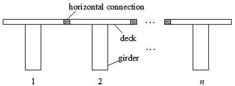
Short-to medium-span bridges are the most widely used types for simply supported bridge in structural design. They can be divided into two categories as integral bridge and multi-girder bridge according to the composition forms of girders. For integral bridge, there is only one piece of girder. Its characteristics of cross section are determined by this girder. For multi-girder one, some horizontal connections between girders are adopted to bear loads as shown in Fig. 1. Its characteristics of cross section are determined comprehensively by the girders.

Fig. 1Sketch for cross section of multi-girder bridge

Assuming each girder in multi-girder bridge possesses the same geometry dimensions, and also the same crack position and depth. Multi-girder bridge can be simplified as integral one for vertical vibration analysis. Equivalent principles are listed as follows:

(a) Height of simplified integral bridge is equal to that of multi-girder one.

(b) Moment of inertia of simplified integral bridge is the sum of values for all girders in multi-girder bridge. It can be expressed as

1

I = \sum_{i = 1}^{n} I_{i},

where $I$ is the moment of inertia of simplified integral bridge, $I_{i}$ is the moment of inertia for $i$ th girder of multi-girder bridge.

(c) Mass per unit length of simplified integral bridge is the sum of values for all girders in multi-girder bridge. It is calculated by:

2

m = \sum_{i = 1}^{n} m_{i},

where $m$ is mass per unit length of simplified integral bridge, $m_{i}$ is mass per unit length for $i$ th girder of multi-girder bridge.

(d) The position and depth of cracks for simplified integral bridge are the same with multi-girder bridge.

Based on above calculation, dynamic analysis of a multi-girder bridge can be simplified as corresponding integral one.

There are several vehicle models, which possesses two degrees of freedom, four degrees of freedom and six degrees of freedom, respectively. In this study, a half-car planar model with four degrees of freedom is adopted.

2.2. Equation of motion and displacement function

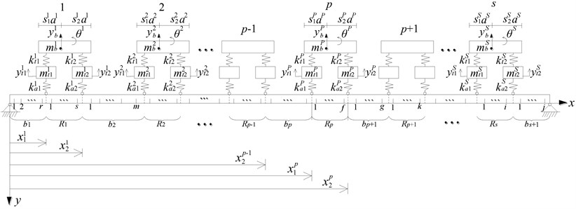
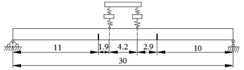
Simply supported bridge with $n$ cracks and under s vehicles is shown in Fig. 2. A half-car planar model is used to simulate the moving vehicle, and 1, 2,…, $p - 1$ , $p$ , $p + 1$ , …, $s$ are vehicle numbers. As shown in Fig. 2, this bridge is divided into ( $2 s + 1$ ) sections by vehicles, which can be expressed by $b_{1}$ , $R_{1}$ , $b_{2}$ , $R_{2}$ , …, $R_{p - 1}$ , $b_{p}$ , $R_{p}$ , $b_{p + 1}$ , $R_{p + 1}$ , …, $R_{s}$ , $b_{s + 1}$ . In each section, there are some cracks and crack numbers are $r$ , $s$ , $m$ ,…, $f$ , $g$ , $k$ ,…, $i$ , $j$ . $m_{b}^{p}$ , $I_{b}^{p}$ and ( $m_{t 1}^{p}$ , $m_{t 2}^{p}$ ) are sprung mass, rotatory mass and wheel mass for the $p$ th vehicle, respectively; $k_{t 1}^{p}$ and $k_{t 2}^{p}$ are suspension spring constants; $k_{a 1}^{p}$ and $k_{a 2}^{p}$ are tyre stiffness coefficients; $a^{P}$ is distance between the left and right wheels of the $p$ th vehicle.

Fig. 2Simply supported bridge with cracks and under multiple vehicles

2.2.1. Equation of motion and displacement function for bridge

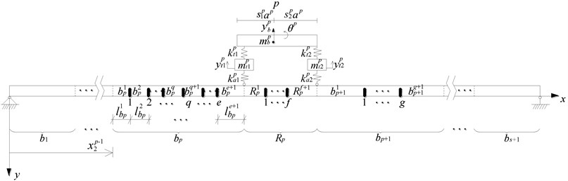
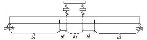
Taking section $b_{p}$ for example, corresponding equation of motion and displacement function are established. Section $b_{p}$ is divided into ( $e + 1$ ) parts by $e$ cracks, which can be denoted by 1, 2,…, $e$ , $e + 1$ , and $l_{b_{p}}^{1}$ , $l_{b_{p}}^{2}$ ,…, $l_{b_{p}}^{e + 1}$ are the lengths of small parts (shown in Fig. 3).

Fig. 3Sketch for division of sections bp, Rp and bp+1

Assuming $ξ = x - (x_{2}^{p - 1} + \sum_{i = 1}^{q - 1} l_{b_{p}}^{i})$ ; for the section $b_{p}^{q}$ , $0 \leq ξ \leq l_{b_{p}}^{q}$ . Equation of motion for section $b_{p}^{q}$ can be established based on Euler-Bernoulli beam theory, which is given by:

3

E I \frac{\partial^{4} y (ξ, t)}{\partial x^{4}} + m \frac{\partial^{2} y (ξ, t)}{\partial t^{2}} = 0,

where $E I$ is flexural rigidity. $E$ is Young’s modulus of bridge, $I$ is moment of inertia, $m$ is mass per unit length. $y (ξ, t)$ is vertical deflection of section $b_{p}^{q}$ at position $ξ$ and time $t$ .

Assuming the whole vibrating system shown in Fig. 2 performs harmonic free vibration at equilibrium position, it has:

4

y (ξ, t) = ϕ_{b_{p}}^{q} (ξ) \cdot e^{j ω t},

where $ω$ is angular frequency for bridge-vehicle system, $ϕ_{b_{p}}^{q} (ξ)$ is corresponding vibration mode function for section $b_{p}^{q}$ .

The substitution of Eq. (4) into Eq. (3) obtains:

5

ϕ_{b_{p}}^{q} (ξ) = A_{b_{p}}^{q} s i n β ξ + B_{b_{p}}^{q} c o s β ξ + C_{b_{p}}^{q} s i n h β ξ + D_{b_{p}}^{q} c o s h β ξ,

where $A_{b_{p}}^{q}$ , $B_{b_{p}}^{q}$ , $C_{b_{p}}^{q}$ , $D_{b_{p}}^{q}$ are undetermined coefficients for section $b_{p}^{q}$ , and $β^{4} = ω^{2} m / E I$ .

2.2.2. Equation of motion and displacement function for vehicle

Equations of motion for wheel masses $m_{t 1}^{p}$ and $m_{t 2}^{p}$ of the $p$ th vehicle are given by:

6

\{\begin{array}{l} m_{t 1}^{p} y_{t 1}^{p} + k_{a 1}^{p} (y_{t 1}^{p} + y_{1}^{p}) + k_{t 1}^{p} (y_{t 1}^{p} - y_{b}^{p} + s_{1}^{p} a^{p} θ^{p}) = 0, \\ m_{t 2}^{p} y_{t 2}^{p} + k_{a 2}^{p} (y_{t 2}^{p} + y_{2}^{p}) + k_{t 2}^{p} (y_{t 2}^{p} - y_{b}^{p} - s_{2}^{p} a^{p} θ^{p}) = 0 . \end{array}

The force balance equations for the $p$ th vehicle body (sprung mass, rotatory mass) are given by:

7

\{\begin{array}{l} m_{b}^{p} y_{b}^{p} + k_{t 1}^{p} (y_{b}^{p} - y_{t 1}^{p} - s_{1}^{p} a^{p} θ^{p}) + k_{t 2}^{p} (y_{b}^{p} - y_{t 2}^{p} + s_{2}^{p} a^{p} θ^{p}) = 0, \\ I_{b}^{p} θ^{p} - s_{1}^{p} a^{p} k_{t 1}^{p} (y_{b}^{p} - y_{t 1}^{p} - s_{1}^{p} a^{p} θ^{p}) + s_{2}^{p} a^{p} k_{t 2}^{p} (y_{b}^{p} - y_{t 2}^{p} + s_{2}^{p} a^{p} θ^{p}) = 0 . \end{array}

The equilibrium equations of motion for the $p$ th vehicle is composed of Eqs. (6-7). $y_{t 1}^{p}$ , $y_{t 2}^{p}$ are deformations for wheel masses $m_{t 1}^{p}$ and $m_{t 2}^{p}$ , respectively; $y_{b}^{p}$ is deformation for sprung mass; $θ^{p}$ is rotation angle for vehicle body; $y_{1}^{p}$ , $y_{2}^{p}$ are deformations at positions $x_{1}^{p}$ and $x_{2}^{p}$ of bridge, respectively.

Because the whole vibrating system performs harmonic free vibration, it can obtain:

8

\{\begin{array}{l} y_{t 1}^{p} = Y_{t 1}^{p} \cdot e^{j ω t}, \\ y_{t 2}^{p} = Y_{t 2}^{p} \cdot e^{j ω t}, \\ y_{b}^{p} = Y_{b}^{p} \cdot e^{j ω t}, \\ θ^{p} = {\hat{θ}}^{p} \cdot e^{j ω t}, \end{array}

where $Y_{t 1}^{p}$ , $Y_{t 2}^{p}$ , $Y_{b}^{p}$ and ${\hat{θ}}^{p}$ are the amplitudes of $y_{t 1}^{p}$ , $y_{t 2}^{p}$ , $y_{b}^{p}$ and $θ^{p}$ respectively. They are undetermined coefficients for amplitudes.

3. Equations of undetermined coefficients

3.1. Equations of bridge sections

Taking section $b_{p}$ for example (shown in Fig. 3), continuity of deformations and equilibrium of moments and forces are satisfied at the right end of $q$ th part and left end of ( $q + 1$ )th part at the $q$ th crack of section $b_{p}$ . It has:

9

\{\begin{array}{l} ϕ_{b_{p}}^{q} (l_{b_{p}}^{q}) = ϕ_{b_{p}}^{q + 1} (0), \\ ϕ_{b_{p}}^{'' q} (l_{b_{p}}^{q}) = ϕ_{b_{p}}^{'' q + 1} (0), \\ ϕ_{b_{p}}^{''' q} (l_{b_{p}}^{q}) = ϕ_{b_{p}}^{''' q + 1} (0) . \end{array}

The slope has a jump at the crack location:

10

ϕ_{b_{p}}^{' q + 1} (0) - ϕ_{b_{p}}^{' q} (l_{b_{p}}^{q}) = θ_{b_{p}}^{q} ϕ_{b_{p}}^{'' q} (l_{b_{p}}^{q}),

11

θ_{b_{p}}^{q} = 5.346 h f (c_{b_{p}}^{q} / h) .

$θ_{b_{p}}^{q}$ is called the flexibility function for open crack. For a rectangular-sectional beam, $f (c_{b_{p}}^{q} / h)$ could be expressed as [30]:

f (c_{b_{p}}^{q} / h) = 1.862 (c_{b_{p}}^{q} / h)^{2} - 3.95 (c_{b_{p}}^{q} / h)^{3} + 16.375 (c_{b_{p}}^{q} / h)^{4} - 37.226 (c_{b_{p}}^{q} / h)^{5}

+ 76.81 (c_{b_{p}}^{q} / h)^{6} - 126 (c_{b_{p}}^{q} / h)^{7} + 172 (c_{b_{p}}^{q} / h)^{8} - 143.97 (c_{b_{p}}^{q} / h)^{9} + 66.56 (c_{b_{p}}^{q} / h)^{10} .

in which $h$ is height of cross-section for bridge at crack position, $c_{b_{p}}^{q}$ is depth of the $q$ th crack in the section $b_{p}$ .

The Eq. (10) can also be applicable for other sections, such as box-girder, circular-sectional beam, etc. Corresponding flexibility function in Eq. (11) varies according to the type of cross-section. In this paper, a numerical example of box-girder is shown in Section 5.3.

The substitutions of Eq. (5) into Eqs. (9-10) obtain:

12

\{\begin{array}{l} B_{b_{p}}^{q + 1} + D_{b_{p}}^{q + 1} = A_{b_{p}}^{q} s i n β l_{b_{p}}^{q} + B_{b_{p}}^{q} c o s β l_{b_{p}}^{q} + C_{b_{p}}^{q} s i n h β l_{b_{p}}^{q} + D_{b_{p}}^{q} c o s h β l_{b_{p}}^{q}, \\ A_{b_{p}}^{q + 1} + C_{b_{p}}^{q + 1} = θ_{b_{p}}^{q} β (- A_{b_{p}}^{q} s i n β l_{b_{p}}^{q} - B_{b_{p}}^{q} c o s β l_{b_{p}}^{q} + C_{b_{p}}^{q} s i n h β l_{b_{p}}^{q} + D_{b_{p}}^{q} c o s h β l_{b_{p}}^{q}) \\ \begin{array}{l}  \end{array} + (A_{b_{p}}^{q} c o s β l_{b_{p}}^{q} - B_{b_{p}}^{q} s i n β l_{b_{p}}^{q} + C_{b_{p}}^{q} c o s h β l_{b_{p}}^{q} + D_{b_{p}}^{q} s i n h β l_{b_{p}}^{q}), \\ - B_{b_{p}}^{q + 1} + D_{b_{p}}^{q + 1} = - A_{b_{p}}^{q} s i n β l_{b_{p}}^{q} - B_{b_{p}}^{q} c o s β l_{b_{p}}^{q} + C_{b_{p}}^{q} s i n h β l_{b_{p}}^{q} + D_{b_{p}}^{q} c o s h β l_{b_{p}}^{q}, \\ - A_{b_{p}}^{q + 1} + C_{b_{p}}^{q + 1} = - A_{b_{p}}^{q} c o s β l_{b_{p}}^{q} + B_{b_{p}}^{q} s i n β l_{b_{p}}^{q} + C_{b_{p}}^{q} c o s h β l_{b_{p}}^{q} + D_{b_{p}}^{q} s i n h β l_{b_{p}}^{q}, \end{array}

or:

13

Z_{b_{p}}^{q + 1} U_{b_{p}}^{q + 1} = Z_{b_{p}}^{q} U_{b_{p}}^{q},

where:

14

U_{b_{p}}^{q} = {\{\begin{array}{l} A_{b_{p}}^{q} & B_{b_{p}}^{q} & C_{b_{p}}^{q} & D_{b_{p}}^{q} \end{array}\}}^{T}, \begin{array}{l}  \end{array} U_{b_{p}}^{q + 1} = {\{\begin{array}{l} A_{b_{p}}^{q + 1} & B_{b_{p}}^{q + 1} & C_{b_{p}}^{q + 1} & D_{b_{p}}^{q + 1} \end{array}\}}^{T},

15

Z_{b_{p}}^{q + 1} = [\begin{matrix} 0 & 1 & 0 & 1 \\ 1 & 0 & 1 & 0 \\ 0 & - 1 & 0 & 1 \\ - 1 & 0 & 1 & 0 \end{matrix}],

16

Z_{b_{p}}^{q} = [\begin{matrix} t_{1} & t_{2} & t_{3} & t_{4} \\ t_{2} - θ_{b_{p}}^{q} β t_{1} & - (t_{1} + θ_{b_{p}}^{q} β t_{2}) & t_{4} + θ_{b_{p}}^{q} β t_{3} & t_{3} + θ_{b_{p}}^{q} β t_{4} \\ - t_{1} & - t_{2} & t_{3} & t_{4} \\ - t_{2} & t_{1} & t_{4} & t_{3} \end{matrix}],

and

t_{1} = s i n β l_{b_{p}}^{q}, t_{2} = c o s β l_{b_{p}}^{q}, t_{3} = s i n h β l_{b_{p}}^{q}, t_{4} = c o s h β l_{b_{p}}^{q}

Eq. (13) can be changed into:

17

U_{b_{p}}^{q + 1} = [Z_{b_{p}}^{q + 1}]^{- 1} Z_{b_{p}}^{q} U_{b_{p}}^{q} = T_{b_{p}}^{q} U_{b_{p}}^{q},

where $T_{b_{p}}^{q}$ is transfer matrix for undetermined coefficients at the right end of $q$ th part and left end of ( $q + 1$ )th part for section $b_{p}$ :

18

T_{b_{p}}^{q} = [\begin{array}{l} t_{11} & t_{12} & t_{13} & t_{14} \\ t_{21} & t_{22} & t_{23} & t_{24} \\ t_{31} & t_{32} & t_{33} & t_{34} \\ t_{41} & t_{42} & t_{43} & t_{44} \end{array}],

where:

t_{11} = c o s β l_{b_{p}}^{q} - \frac{1}{2} θ_{b_{p}}^{q} β s i n β l_{b_{p}}^{q}, t_{12} = - s i n β l_{b_{p}}^{q} - \frac{1}{2} θ_{b_{p}}^{q} β c o s β l_{b_{p}}^{q},

t_{13} = \frac{1}{2} θ_{b_{p}}^{q} β s i n h β l_{b_{p}}^{q}, t_{14} = \frac{1}{2} θ_{b_{p}}^{q} β c o s h β l_{b_{p}}^{q},

t_{21} = s i n β l_{b_{p}}^{q}, \begin{array}{l}  \end{array} t_{22} = c o s β l_{b_{p}}^{q}, \begin{array}{l}  \end{array} t_{23} = 0, \begin{array}{l}  \end{array} t_{24} = 0,

t_{31} = - \frac{1}{2} θ_{b_{p}}^{q} β s i n β l_{b_{p}}^{q}, t_{32} = - \frac{1}{2} θ_{b_{p}}^{q} β c o s β l_{b_{p}}^{q},

t_{33} = c o s h β l_{b_{p}}^{q} + \frac{1}{2} θ_{b_{p}}^{q} β s i n h β l_{b_{p}}^{q}, t_{34} = s i n h β l_{b_{p}}^{q} + \frac{1}{2} θ_{b_{p}}^{q} β c o s h β l_{b_{p}}^{q},

t_{41} = 0, \begin{array}{l}  \end{array} t_{42} = 0, \begin{array}{l}  \end{array} t_{43} = s i n h β l_{b_{p}}^{q}, \begin{array}{l}  \end{array} t_{44} = c o s h β l_{b_{p}}^{q} .

The transfer relationship from the 1st part to ( $e + 1$ )th part in section $b_{p}$ can be given by:

19

U_{b_{p}}^{e + 1} = T_{b_{p}}^{e} T_{b_{p}}^{e - 1} \cdot \cdot \cdot T_{b_{p}}^{2} T_{b_{p}}^{1} U_{b_{p}}^{1} .

Assuming:

20

T_{b_{p}} = T_{b_{p}}^{e} T_{b_{p}}^{e - 1} \cdot \cdot \cdot T_{b_{p}}^{2} T_{b_{p}}^{1} .

Eq. (19) can be expressed by:

21

U_{b_{p}}^{e + 1} = T_{b_{p}} U_{b_{p}}^{1},

where $T_{b_{p}}$ is transfer matrix for undetermined coefficients of section $b_{p}$ . If section $b_{p}$ has no crack, division is not necessary. One group of underdetermined coefficients is able to represent the mode function. In order to obtain the uniform representation of coefficients in each section, Eq. (21) is also used to represent its coefficient equation even if the section of $b_{p}$ has no crack. Here, $U_{b_{p}}^{e + 1}$ has the same meaning with $U_{b_{p}}^{1}$ , and $T_{b_{p}}$ is identity matrix.

3.2. Equations at wheels

As shown in Fig. 3, sections $b_{p}$ , $R_{p}$ and $b_{p + 1}$ are divided into ( $e + 1$ ), ( $f + 1$ ) and ( $g + 1$ ) parts, respectively. The last parts for $b_{p}$ , $R_{p}$ and $b_{p + 1}$ can be denoted by $b_{p}^{e + 1}$ , $R_{p}^{f + 1}$ and $b_{p + 1}^{g + 1}$ , while their lengths are $l_{b_{p}}^{e + 1}$ , $l_{R_{p}}^{f + 1}$ and $l_{b_{p + 1}}^{g + 1}$ . $ϕ_{b_{p}}^{1}$ , $ϕ_{R_{p}}^{1}$ and $ϕ_{b_{p + 1}}^{1}$ are used to represent the mode functions of the first part for sections $b_{p}$ , $R_{p}$ and $b_{p + 1}$ . $ϕ_{b_{p}}^{e + 1}$ , $ϕ_{R_{p}}^{f + 1}$ and $ϕ_{b_{p + 1}}^{g + 1}$ are used to represent the mode functions of the last part for sections $b_{p}$ , $R_{p}$ and $b_{p + 1}$ .

Continuity of deformations and equilibrium of moments and forces are satisfied at the position of left wheel of the $p$ th vehicle ( $x_{1}^{p}$ ), it has:

22

\{\begin{array}{l} ϕ_{b_{p}}^{e + 1} (l_{b_{p}}^{e + 1}) = ϕ_{R_{p}}^{1} (0), \\ ϕ_{b_{p}}^{' e + 1} (l_{b_{p}}^{e + 1}) + {W_{L}}_{b_{p}}^{e + 1} = ϕ_{R_{p}}^{' 1} (0), \\ ϕ_{b_{p}}^{'' e + 1} (l_{b_{p}}^{e + 1}) = ϕ_{R_{p}}^{'' 1} (0), \\ E I ϕ_{b_{p}}^{''' e + 1} (l_{b_{p}}^{e + 1}) - ω^{2} m_{t 1}^{p} Y_{t 1}^{p} + k_{t 1}^{p} (Y_{t 1}^{p} - Y_{b}^{p} + s_{1}^{p} a^{p} {\hat{θ}}^{p}) - E I ϕ_{R_{p}}^{''' 1} (0) = 0 . \end{array}

The substitution of Eq. (5) into Eq. (22), it has:

23

\{\begin{array}{l} B_{R_{p}}^{1} + D_{R_{p}}^{1} = A_{b_{p}}^{e + 1} s i n β l_{b_{p}}^{e + 1} + B_{b_{p}}^{e + 1} c o s β l_{b_{p}}^{e + 1} + C_{b_{p}}^{e + 1} s i n h β l_{b_{p}}^{e + 1} + D_{b_{p}}^{e + 1} c o s h β l_{b_{p}}^{e + 1}, \\ A_{R_{p}}^{1} + C_{R_{p}}^{1} = A_{b_{p}}^{e + 1} c o s β l_{b_{p}}^{e + 1} + B_{b_{p}}^{e + 1} s i n β l_{b_{p}}^{e + 1} + C_{b_{p}}^{e + 1} c o s h β l_{b_{p}}^{e + 1} + D_{b_{p}}^{e + 1} s i n h β l_{b_{p}}^{e + 1} + {W_{L}}_{b_{p}}^{e + 1}, \\ - B_{R_{p}}^{1} + D_{R_{p}}^{1} = - A_{b_{p}}^{e + 1} s i n β l_{b_{p}}^{e + 1} - B_{b_{p}}^{e + 1} c o s β l_{b_{p}}^{e + 1} + C_{b_{p}}^{e + 1} s i n h β l_{b_{p}}^{e + 1} + D_{b_{p}}^{e + 1} c o s h β l_{b_{p}}^{e + 1}, \\ - A_{R_{p}}^{1} + C_{R_{p}}^{1} = (- A_{b_{p}}^{e + 1} c o s β l_{b_{p}}^{e + 1} + B_{b_{p}}^{e + 1} s i n β l_{b_{p}}^{e + 1} + C_{b_{p}}^{e + 1} c o s h β l_{b_{p}}^{e + 1} + D_{b_{p}}^{e + 1} s i n h β l_{b_{p}}^{e + 1}) \\ \begin{array}{l}  \end{array} - [ω^{2} m_{t 1}^{p} Y_{t 1}^{p} - k_{t 1}^{p} (Y_{t 1}^{p} - Y_{b}^{p} + s_{1}^{p} a^{p} {\hat{θ}}^{p})] / E I β^{3}, \end{array}

where $A_{b_{p}}^{e + 1}$ , $B_{b_{p}}^{e + 1}$ , $C_{b_{p}}^{e + 1}$ and $D_{b_{p}}^{e + 1}$ are undetermined coefficients for the last part (( $e + 1$ )th part) of section $b_{p}$ , while $A_{R_{p}}^{1}$ , $B_{R_{p}}^{1}$ , $C_{R_{p}}^{1}$ and $D_{R_{p}}^{1}$ are coefficients for the first part of $R_{p}$ . ${W_{L}}_{b_{p}}^{e + 1} = θ_{b_{p}}^{e + 1} β (- A_{b_{p}}^{e + 1} s i n β l_{b_{p}}^{e + 1} - B_{b_{p}}^{e + 1} c o s β l_{b_{p}}^{e + 1} + C_{b_{p}}^{e + 1} s i n h β l_{b_{p}}^{e + 1} + D_{b_{p}}^{e + 1} c o s h β l_{b_{p}}^{e + 1})$ .

Eq. (23) can be represented by matrix form, it is:

24

[H^{p L}] \{U^{p L}\} = [\begin{array}{l} H_{1}^{p L} & \begin{array}{l} H_{2}^{p L} & H_{3}^{p L} \end{array} \end{array}] \{\begin{matrix} U_{b_{p}}^{e + 1} \\ U_{R_{p}}^{1} \\ U_{v}^{p} \end{matrix}\} = 0,

here:

25

[H_{1}^{p L}] = [\begin{matrix} s i n β l_{b_{p}}^{e + 1} & c o s β l_{b_{p}}^{e + 1} & s i n h β l_{b_{p}}^{e + 1} & c o s h β l_{b_{p}}^{e + 1} \\ c o s β l_{b_{p}}^{e + 1} + {W_{L}}_{1} & - s i n β l_{b_{p}}^{e + 1} + {W_{L}}_{2} & c o s h β l_{b_{p}}^{e + 1} + {W_{L}}_{3} & s i n h β l_{b_{p}}^{e + 1} + {W_{L}}_{4} \\ - s i n β l_{b_{p}}^{e + 1} & - c o s β l_{b_{p}}^{e + 1} & s i n h β l_{b_{p}}^{e + 1} & c o s h β l_{b_{p}}^{e + 1} \\ - E I β^{3} c o s β l_{b_{p}}^{e + 1} & E I β^{3} s i n β l_{b_{p}}^{e + 1} & E I β^{3} c o s h β l_{b_{p}}^{e + 1} & E I β^{3} s i n h β l_{b_{p}}^{e + 1} \end{matrix}],

26

[\begin{array}{l} H_{2}^{p L} & H_{3}^{p L} \end{array}] = [\begin{matrix} 0 & - 1 & 0 & - 1 & 0 & 0 & 0 & 0 \\ - 1 & 0 & - 1 & 0 & 0 & 0 & 0 & 0 \\ 0 & 1 & 0 & - 1 & 0 & 0 & 0 & 0 \\ E I β^{3} & 0 & - E I β^{3} & 0 & - ω^{2} m_{t 1}^{p} + k_{t 1}^{p} & 0 & - k_{t 1}^{p} & s_{1}^{p} a^{p} k_{t 1}^{p} \end{matrix}],

27

\{U_{b_{p}}^{e + 1}\} = {\{\begin{array}{l} A_{b_{p}}^{e + 1} & B_{b_{p}}^{e + 1} & C_{b_{p}}^{e + 1} & D_{b_{p}}^{e + 1} \end{array}\}}^{T},

\{U_{R_{p}}^{1}\} = {\{\begin{array}{l} A_{R_{p}}^{1} & B_{R_{p}}^{1} & C_{R_{p}}^{1} & D_{R_{p}}^{1} \end{array}\}}^{T},

\{U_{v}^{p}\} = {\{\begin{array}{l} Y_{t 1}^{p} & Y_{t 2}^{p} & Y_{b}^{p} & {\hat{θ}}^{p} \end{array}\}}^{T},

{W_{L}}_{1} = - θ_{b_{p}}^{e + 1} β s i n β l_{b_{p}}^{e + 1}, {W_{L}}_{2} = - θ_{b_{p}}^{e + 1} β c o s β l_{b_{p}}^{e + 1},

{W_{L}}_{3} = θ_{b_{p}}^{e + 1} β s i n h β l_{b_{p}}^{e + 1}, {W_{L}}_{4} = θ_{b_{p}}^{e + 1} β c o s h β l_{b_{p}}^{e + 1} .

When the left wheel is just at the crack position, ${W_{L}}_{b_{p}}^{e + 1}$ , ${W_{L}}_{1}$ , ${W_{L}}_{2}$ , ${W_{L}}_{3}$ and ${W_{L}}_{4}$ are not equal to zero; on the contrary, ${W_{L}}_{b_{p}}^{e + 1}$ , ${W_{L}}_{1}$ , ${W_{L}}_{2}$ , ${W_{L}}_{3}$ and ${W_{L}}_{4}$ are equal to zero.

The substitution of Eq. (21) into Eq. (24), it has:

28

[H^{p L}] \{U^{p L}\} = [\begin{array}{l} H_{1}^{p L} T_{b_{p}} & \begin{array}{l} H_{2}^{p L} & H_{3}^{p L} \end{array} \end{array}] \{\begin{matrix} U_{b_{p}}^{1} \\ U_{R_{p}}^{1} \\ U_{v}^{p} \end{matrix}\} = 0,

where $\{U_{b_{p}}^{1}\} = {\{\begin{array}{l} A_{b_{p}}^{1} & B_{b_{p}}^{1} & C_{b_{p}}^{1} & D_{b_{p}}^{1} \end{array}\}}^{T}$ , which is the undetermined coefficient vector for mode shape of the first part of section $b_{p}$ ; $T_{b_{p}}$ is transfer matrix for undetermined coefficients of section $b_{p}$ .

At the right wheel of $p$ th vehicle ( $x_{2}^{p}$ ), it can also obtain that:

29

\{\begin{array}{l} B_{b_{p + 1}}^{1} + D_{b_{p + 1}}^{1} = A_{R_{p}}^{f + 1} s i n β l_{R_{p}}^{f + 1} + B_{R_{p}}^{f + 1} c o s β l_{R_{p}}^{f + 1} \\ + C_{R_{p}}^{f + 1} s i n h β l_{R_{p}}^{f + 1} + D_{R_{p}}^{f + 1} c o s h β l_{R_{p}}^{f + 1}, \\ A_{b_{p + 1}}^{1} + C_{b_{p + 1}}^{1} = A_{R_{p}}^{f + 1} c o s β l_{R_{p}}^{f + 1} + B_{R_{p}}^{f + 1} s i n β l_{R_{p}}^{f + 1} \\ + C_{R_{p}}^{f + 1} c o s h β l_{R_{p}}^{f + 1} + D_{R_{p}}^{f + 1} s i n h β l_{R_{p}}^{f + 1} + {W_{R}}_{R_{p}}^{f + 1}, \\ - B_{b_{p + 1}}^{1} + D_{b_{p + 1}}^{1} = - A_{R_{p}}^{f + 1} s i n β l_{R_{p}}^{f + 1} - B_{R_{p}}^{f + 1} c o s β l_{R_{p}}^{f + 1} \\ + C_{R_{p}}^{f + 1} s i n h β l_{R_{p}}^{f + 1} + D_{R_{p}}^{f + 1} c o s h β l_{R_{p}}^{f + 1}, \\ - A_{b_{p + 1}}^{1} + C_{b_{p + 1}}^{1} = (- A_{R_{p}}^{f + 1} c o s β l_{R_{p}}^{f + 1} + B_{R_{p}}^{f + 1} s i n β l_{R_{p}}^{f + 1} + C_{R_{p}}^{f + 1} c o s h β l_{R_{p}}^{f + 1} \\ + D_{R_{p}}^{f + 1} s i n h β l_{R_{p}}^{f + 1}) - [ω^{2} m_{t 2}^{p} Y_{t 2}^{p} - k_{t 2}^{p} (Y_{t 2}^{p} - Y_{b}^{p} + s_{2}^{p} a^{p} {\hat{θ}}^{p})] / E I β^{3} . \end{array}

Eq. (29) can be represented by matrix form, it is:

30

[H^{p R}] \{U^{p R}\} = [\begin{array}{l} H_{1}^{p R} & \begin{array}{l} H_{2}^{p R} & H_{3}^{p R} \end{array} \end{array}] \{\begin{matrix} U_{R_{p}}^{f + 1} \\ U_{v}^{p} \\ U_{b_{p + 1}}^{1} \end{matrix}\} = 0,

here:

31

[H_{1}^{p R}] = [\begin{matrix} s i n β l_{R_{p}}^{f + 1} & c o s β l_{R_{p}}^{f + 1} & s i n h β l_{R_{p}}^{f + 1} & c o s h β l_{R_{p}}^{f + 1} \\ c o s β l_{R_{p}}^{f + 1} + {W_{R}}_{1} & - s i n β l_{R_{p}}^{f + 1} + {W_{R}}_{2} & c o s h β l_{R_{p}}^{f + 1} + {W_{R}}_{3} & s i n h β l_{R_{p}}^{f + 1} + {W_{R}}_{4} \\ - s i n β l_{R_{p}}^{f + 1} & - c o s β l_{R_{p}}^{f + 1} & s i n h β l_{R_{p}}^{f + 1} & c o s h β l_{R_{p}}^{f + 1} \\ - E I β^{3} c o s β l_{R_{p}}^{f + 1} & E I β^{3} s i n β l_{R_{p}}^{f + 1} & E I β^{3} c o s h β l_{R_{p}}^{f + 1} & E I β^{3} s i n h β l_{R_{p}}^{f + 1} \end{matrix}],

32

[\begin{array}{l} H_{2}^{p R} & H_{3}^{p R} \end{array}] = [\begin{array}{l} 0 & 0 & 0 & 0 & 0 & - 1 & 0 & - 1 \\ 0 & 0 & 0 & 0 & - 1 & 0 & - 1 & 0 \\ 0 & 0 & 0 & 0 & 0 & 1 & 0 & - 1 \\ 0 & - ω^{2} m_{t 2}^{p} + k_{t 2}^{p} & - k_{t 2}^{p} & - s_{2}^{p} a^{p} k_{t 2}^{p} & E I β^{3} & 0 & - E I β^{3} & 0 \end{array}],

33

\{U_{R_{p}}^{f + 1}\} = {\{\begin{array}{l} A_{R_{p}}^{f + 1} & B_{R_{p}}^{f + 1} & C_{R_{p}}^{f + 1} & D_{R_{p}}^{f + 1} \end{array}\}}^{T}, \{U_{v}^{p}\} = {\{\begin{array}{l} Y_{t 1}^{p} & Y_{t 2}^{p} & Y_{b}^{p} & {\hat{θ}}^{p} \end{array}\}}^{T},

\{U_{b_{p + 1}}^{1}\} = {\{\begin{array}{l} A_{b_{p + 1}}^{1} & B_{b_{p + 1}}^{1} & C_{b_{p + 1}}^{1} & D_{b_{p + 1}}^{1} \end{array}\}}^{T},

{W_{R}}_{R_{p}}^{f + 1} = θ_{R_{p}}^{f + 1} β (- A_{R_{p}}^{f + 1} s i n β l_{R_{p}}^{f + 1} - B_{R_{p}}^{f + 1} c o s β l_{R_{p}}^{f + 1} + C_{R_{p}}^{f + 1} s i n h β l_{R_{p}}^{f + 1} + D_{R_{p}}^{f + 1} c o s h β l_{R_{p}}^{f + 1}),

{W_{R}}_{1} = - θ_{R_{p}}^{f + 1} β s i n β l_{R_{p}}^{f + 1}, {W_{R}}_{2} = - θ_{R_{p}}^{f + 1} β c o s β l_{R_{p}}^{f + 1},

{W_{R}}_{3} = θ_{R_{p}}^{f + 1} β s i n h β l_{R_{p}}^{f + 1}, {W_{R}}_{4} = θ_{R_{p}}^{f + 1} β c o s h β l_{R_{p}}^{f + 1} .

When the right wheel is just at the crack position, ${W_{R}}_{R_{p}}^{f + 1}$ , ${W_{R}}_{1}$ , ${W_{R}}_{2}$ , ${W_{R}}_{3}$ and ${W_{R}}_{4}$ are not equal to zero; on the contrary, ${W_{R}}_{R_{p}}^{f + 1}$ , ${W_{R}}_{1}$ , ${W_{R}}_{2}$ , ${W_{R}}_{3}$ and ${W_{R}}_{4}$ are equal to zero.

The substitution of Eq. (21) into Eq. (30), it has:

34

[H^{p R}] \{U^{p R}\} = [\begin{array}{l} H_{1}^{p R} T_{R_{p}} & \begin{array}{l} H_{2}^{p R} & H_{3}^{p R} \end{array} \end{array}] \{\begin{matrix} U_{R_{p}}^{1} \\ U_{v}^{p} \\ U_{b_{p + 1}}^{1} \end{matrix}\} = 0,

where $T_{R_{p}}$ is transfer matrix for undetermined coefficients of section $R_{p}$ .

3.3. Equations from motion of vehicles

The substitutions of Eqs. (4-5, 8) into Eqs. (6-7), one obtains:

35

\{\begin{array}{l} k_{a 1}^{p} (B_{R_{p}}^{1} + D_{R_{p}}^{1}) - ω^{2} m_{t 1}^{p} Y_{t 1}^{p} + k_{a 1}^{p} Y_{t 1}^{p} + k_{t 1}^{p} (Y_{t 1}^{p} - Y_{b}^{p} + s_{1}^{p} a^{p} {\hat{θ}}^{p}) = 0, \\ k_{a 2}^{p} (B_{b_{p + 1}}^{1} + D_{b_{p + 1}}^{1}) - ω^{2} m_{t 2}^{p} Y_{t 2}^{p} + k_{a 2}^{p} Y_{t 2}^{p} + k_{t 2}^{p} (Y_{t 2}^{p} - Y_{b}^{p} - s_{2}^{p} a^{p} {\hat{θ}}^{p}) = 0, \\ - ω^{2} m_{b}^{p} Y_{b}^{p} + k_{t 1}^{p} (Y_{b}^{p} - Y_{t 1}^{p} - s_{1}^{p} a^{p} {\hat{θ}}^{p}) + k_{t 2}^{p} (Y_{b}^{p} - Y_{t 2}^{p} + s_{2}^{p} a^{p} {\hat{θ}}^{p}) = 0, \\ - ω^{2} I_{b}^{p} {\hat{θ}}^{p} - s_{1}^{p} a^{p} k_{t 1}^{p} (Y_{b}^{p} - Y_{t 1}^{p} - s_{1}^{p} a^{p} {\hat{θ}}^{p}) + s_{2}^{p} a^{p} k_{t 2}^{p} (Y_{b}^{p} - Y_{t 2}^{p} + s_{2}^{p} a^{p} {\hat{θ}}^{p}) = 0, \end{array}

or:

36

[H^{p V}] \{U^{p V}\} = [\begin{array}{l} H_{1}^{p V} & \begin{array}{l} H_{2}^{p V} & H_{3}^{p V} \end{array} \end{array}] \{\begin{matrix} U_{R_{p}}^{1} \\ U_{v}^{p} \\ U_{b_{p + 1}}^{1} \end{matrix}\} = 0,

where:

37

[H_{1}^{p V}] = [\begin{array}{l} 0 & k_{a 1}^{p} & 0 & k_{a 1}^{p} \\ 0 & 0 & 0 & 0 \\ 0 & 0 & 0 & 0 \\ 0 & 0 & 0 & 0 \end{array}],

38

[H_{2}^{p V}]

= [\begin{matrix} - ω^{2} m_{t 1}^{p} + k_{a 1}^{p} + k_{t 1}^{p} & 0 & - k_{t 1}^{p} & s_{1}^{p} a^{p} k_{t 1}^{p} \\ 0 & - ω^{2} m_{t 2}^{p} + k_{a 2}^{p} + k_{t 2}^{p} & - k_{t 2}^{p} & - s_{2}^{p} a^{p} k_{t 2}^{p} \\ - k_{t 1}^{p} & - k_{t 2}^{p} & - ω^{2} m_{b}^{p} + k_{t 1}^{p} + k_{t 2}^{p} & s_{2}^{p} a^{p} k_{t 2}^{p} - s_{1}^{p} a^{p} k_{t 1}^{p} \\ s_{1}^{p} a^{p} k_{t 1}^{p} & - s_{2}^{p} a^{p} k_{t 2}^{p} & s_{2}^{p} a^{p} k_{t 2}^{p} - s_{1}^{p} a^{p} k_{t 1}^{p} & - ω^{2} I_{b}^{p} + {(a^{p})}^{2} ({(s_{2}^{p})}^{2} k_{t 2}^{p} + {(s_{1}^{p})}^{2} k_{t 1}^{p}) \end{matrix}],

39

[H_{3}^{p V}] = [\begin{array}{l} 0 & 0 & 0 & 0 \\ 0 & k_{a 2}^{p} & 0 & k_{a 2}^{p} \\ 0 & 0 & 0 & 0 \\ 0 & 0 & 0 & 0 \end{array}] .

3.4. Equations from boundary conditions

At the left end, displacement and moment are zero, and it has:

40

\{\begin{array}{l} ϕ_{b_{1}}^{1} (0) = 0, \\ ϕ_{b_{1}}^{'' 1} (0) = 0, \end{array}

where $ϕ_{b_{1}}^{1}$ is mode function for the first part of section $b_{1}$ .

The substitution of Eq. (5) into Eq. (40), one obtains:

41

\{\begin{array}{l} B_{b_{1}}^{1} + D_{b_{1}}^{1} = 0, \\ - B_{b_{1}}^{1} + D_{b_{1}}^{1} = 0, \end{array}

or:

42

[H_{s 1}] \{U_{b_{1}}^{1}\} = 0,

where:

43

[H_{s 1}] = [\begin{array}{l} 0 & 1 & 0 & 1 \\ 0 & - 1 & 0 & 1 \end{array}],

44

\{U_{b_{1}}^{1}\} = {\{\begin{array}{l} A_{b_{1}}^{1} & B_{b_{1}}^{1} & C_{b_{1}}^{1} & D_{b_{1}}^{1} \end{array}\}}^{T} .

$A_{b_{1}}^{1}$ , $B_{b_{1}}^{1}$ , $C_{b_{1}}^{1}$ and $D_{b_{1}}^{1}$ are undetermined coefficients for mode shape of the first part of section $b_{1}$ .

Section $b_{s + 1}$ is divided into ( $j + 1$ ) parts, the length for ( $j + 1$ )th part is $l_{b_{s + 1}}^{j + 1}$ . According to the boundary condition of right end of bridge, it has:

45

\{\begin{array}{l} ϕ_{b_{s + 1}}^{j + 1} (l_{b_{s + 1}}^{j + 1}) = 0, \\ ϕ_{b_{s + 1}}^{'' j + 1} (l_{b_{s + 1}}^{j + 1}) = 0 . \end{array}

The substitution of Eq. (5) into Eq. (45), one obtains:

46

\{\begin{array}{l} A_{b_{s + 1}}^{j + 1} s i n β l_{b_{s + 1}}^{j + 1} + B_{b_{s + 1}}^{j + 1} c o s β l_{b_{s + 1}}^{j + 1} + C_{b_{s + 1}}^{j + 1} s i n h β l_{b_{s + 1}}^{j + 1} + D_{b_{s + 1}}^{j + 1} c o s h β l_{b_{s + 1}}^{j + 1} = 0, \\ - A_{b_{s + 1}}^{j + 1} s i n β l_{b_{s + 1}}^{j + 1} - B_{b_{s + 1}}^{j + 1} c o s β l_{b_{s + 1}}^{j + 1} + C_{b_{s + 1}}^{j + 1} s i n h β l_{b_{s + 1}}^{j + 1} + D_{b_{s + 1}}^{j + 1} c o s h β l_{b_{s + 1}}^{j + 1} = 0, \end{array}

where $A_{b_{s + 1}}^{j + 1}$ , $B_{b_{s + 1}}^{j + 1}$ , $C_{b_{s + 1}}^{j + 1}$ and $D_{b_{s + 1}}^{j + 1}$ are undetermined coefficients for mode shape of the ( $j + 1$ )th part of section $b_{s + 1}$ .

Eq. (46) is represented by matrix form, it obtains:

47

[H_{s 2}] \{U_{b_{s + 1}}^{j + 1}\} = 0,

where:

48

[H_{s 2}] = [\begin{matrix} s i n β l_{b_{s + 1}}^{j + 1} & c o s β l_{b_{s + 1}}^{j + 1} & s i n h β l_{b_{s + 1}}^{j + 1} & c o s h β l_{b_{s + 1}}^{j + 1} \\ - s i n β l_{b_{s + 1}}^{j + 1} & - c o s β l_{b_{s + 1}}^{j + 1} & s i n h β l_{b_{s + 1}}^{j + 1} & c o s h β l_{b_{s + 1}}^{j + 1} \end{matrix}],

49

\{U_{b_{s + 1}}^{j + 1}\} = \{\begin{array}{l} A_{b_{s + 1}}^{j + 1} & B_{b_{s + 1}}^{j + 1} & C_{b_{s + 1}}^{j + 1} & D_{b_{s + 1}}^{j + 1} \end{array}\} .

The substitution of Eq. (21) into Eq. (47), one obtains:

50

[H_{s 2}] [T_{b_{s + 1}}] \{U_{b_{s + 1}}^{1}\} = 0,

51

\{U_{b_{s + 1}}^{1}\} = {\{\begin{array}{l} A_{b_{s + 1}}^{1} & B_{b_{s + 1}}^{1} & C_{b_{s + 1}}^{1} & D_{b_{s + 1}}^{1} \end{array}\}}^{T},

where $A_{b_{s + 1}}^{1}$ , $B_{b_{s + 1}}^{1}$ , $C_{b_{s + 1}}^{1}$ and $D_{b_{s + 1}}^{1}$ are undetermined coefficients for mode shape of the first part of section $b_{s + 1}$ ; $T_{b_{s + 1}}$ is transfer matrix for coefficients of section $b_{s + 1}$ .

4. Determination of natural frequencies and modal shapes

For cracked simply supported bridge under s vehicles (shown in Fig. 2), the bridge is divided into $2 s + 1$ sections by vehicles, which can be represented by $b_{1}$ , $R_{1}$ , $b_{2}$ , $R_{2}$ … $R_{p - 1}$ , $b_{p}$ , $R_{p}$ , $b_{p + 1}$ , $R_{p + 1}$ ,…, $R_{s}$ , $b_{s + 1}$ . At one section, undetermined coefficients of mode shape for each part can be represented by four coefficients of the first part (shown in Eq. (21)). Therefore, there are four undetermined coefficients for each section. For $2 s + 1$ sections, there are totally $4 \times (2 s + 1)$ coefficients. Moreover, there are four undetermined coefficients for each vehicle. The whole system possesses $4 \times (2 s + 1) + 4 \times s = 12 s + 4$ undetermined coefficients.

There are four equations for undetermined coefficients at the left wheel of vehicle (shown in Eq. (28)); and four equations for undetermined coefficients at the right wheel of vehicle (shown in Eq. (34)). Four equations for coefficients can be obtained by equation of motion of vehicle (shown in Eq. (36)). Therefore, there are totally twelve equations for each vehicle, and $12 s$ equations for $s$ vehicles. At the left end and right end of bridge, there are two equations for undetermined coefficients, respectively (shown in Eqs. (42, 50)). In general, there are totally $12 s + 4$ equations for undetermined coefficients. Numerical assembly method is adopted to obtain the matrix equation of all undetermined coefficients, one has:

52

[H] {U} = 0,

where:

53

[H] = \begin{matrix} \begin{matrix} 1 \to 4 & \dots & n + 1 \to & n + 5 \to & n + 9 \to & n + 13 \to & \dots & n^{'} + 1 \to \\ n + 4 & n + 8 & n + 12 & n + 16 & n^{'} + 4 \end{matrix} \\ [\begin{matrix} H_{s 1} \\ ⋱ \\ H_{1}^{p L} T_{b_{p}} & H_{2}^{p L} & H_{3}^{p L} \\ H_{1}^{p R} T_{R_{p}} & H_{2}^{p R} & H_{3}^{p R} \\ H_{1}^{p V} & H_{2}^{p V} & H_{3}^{p V} \\ ⋱ \\ H_{s 2} T_{b_{s + 1}} \end{matrix}] & \begin{matrix} 1 \to 2 \\ \dots \\ m + 1 \to m + 4 \\ m + 5 \to m + 8 \\ m + 9 \to m + 12 \\ \dots \\ m' + 1 \to m^{'} + 2 \end{matrix} \end{matrix}

54

\begin{matrix} \begin{array}{l} 1 \end{array} \to \begin{array}{l} 4 \end{array} & n + 1 \to & n + 5 \to & n + 9 \to & n + 13 \to & n' + 1 \to \\ n + 4 & n + 8 & n + 12 & n + 16 & n' + 4 \\ \{U\} = & {U_{b_{1}}^{1} & U_{b_{p}}^{1} & U_{R_{p}}^{1} & U_{V} & U_{b_{p + 1}}^{1} & U_{b_{S + 1}}^{1}}, \end{matrix}

55

\{\begin{array}{l} m = 12 (p - 1) + 2, \\ n = 4 (2 (p - 1) + (p - 1)) = 12 (p - 1), \\ m' = 12 s + 2, \\ n^{'} = 4 (2 s + s) = 12 s, \end{array}

here, $p$ , $s$ are vehicle numbers.

In the process of assembling matrix [H], position for each element can be determined by identification number shown at the right side and top of matrix shown in Eq. (53). Identification numbers for undetermined coefficients are shown in Eq. (54).

Non-trivial solution of Eq. (52) requires that:

56

|H| = 0 .

Half-interval method is used to determine the natural frequencies $ω_{i}$ ( $i =$ 1, 2, ...) of cracked simply supported bridge under multiple vehicles. For each order of natural frequency, it satisfies Eq. (56). Mode shapes can be obtained by substituting natural frequencies $ω_{i}$ ( $i =$ 1, 2, ...) into Eq. (5). The detailed process for determining lowest natural frequencies is as follows: Firstly, an initial value of frequency coefficient $ω_{a}$ is assumed, the values of coefficient matrix $|H|$ corresponding to $ω_{a}$ are obtained and the values of $|H|$ are calculated, $D_{a} = |H_{ω_{a}}|$ . Then a new value $ω_{b} = ω_{a} + ∆ ω$ with $∆ ω$ (e.g. $∆ ω =$ 0.5) representing the increment of $ω$ is assumed, and the same calculations are repeated to determine the new value of determinant corresponding to $ω_{b}$ , $D_{b} = |H_{ω_{b}}|$ . If $D_{a}$ and $D_{b}$ have opposite signs, there is at least one frequency coefficient in the interval [ $ω_{a}$ , $ω_{b}$ ]; if $D_{a}$ and $D_{b}$ have the same sign, let $ω_{a} = ω_{b}$ , it needs to continue the above procedure until $D_{a}$ and $D_{b}$ have opposite signs. For the next step, let $ω_{c} = (ω_{a} + ω_{b}) / 2$ , if $D_{a}$ and $D_{c}$ have the same sign, let $ω_{a} = ω_{c}$ ; if $D_{a}$ and $D_{c}$ have opposite signs, $ω_{b} = ω_{c}$ , a new interval [ $ω_{a}$ , $ω_{b}$ ] is obtained. The same calculations are repeated to determine the new interval [ $ω_{a}$ , $ω_{b}$ ] until the rank of matrix $|H|$ is equal to $q - 1$ . The accurate values of $ω$ are obtained respectively using the half-interval method. The substitution of the obtained frequency $ω$ into Eq. (5) will determine the corresponding mode shape of the bridge.

5. Numerical simulation and discussions

5.1. Reliability of the proposed method

5.1.1. Cracked simply supported beam without vehicle

In order to illustrate the proposed method, numerical example will show how to determine the natural frequencies of a simply supported beam with uniform cross-section and with cracks.

Structural parameters [31]: length $L =$ 800 mm, width = 10 mm, height = 60 mm, Young’s modulus $E =$ 2.0×10¹¹ Pa, mass density $ρ =$ 7.8×10³ kg/m³.

The first two order natural frequencies are obtained through the proposed method in this paper. Corresponding reduction coefficient $η$ is calculated by Eq. (57), which can be used to demonstrate the effect of crack on natural frequencies of simply supported beam without vehicle:

57

η_{j} = \frac{ω_{c j}}{ω_{j}},

where $ω_{c j}$ and $ω_{j}$ are the $j$ th natural frequency of the cracked and un-cracked beams, respectively, $η_{j}$ is the reduction coefficient of the $j$ th natural frequency.

In this paper, four different crack depths ( $c =$ 10, 15, 20 and 25 mm) at four different locations ( $x_{1} =$ 100, 200, 300 and 400 mm, $x_{1}$ is the distance between crack location and the left end of the beam) are investigated. Corresponding $η_{1}$ and $η_{2}$ are calculated and shown in Fig. 4. The results obtained by Liang et al. [31] are also presented in Fig. 4, which are denoted by “·”.

Fig. 4Crack-induced eigen-frequency changes for various crack locations and depths

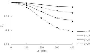
a) Reduction coefficient for 1st natural frequency ( $η_{1}$ )

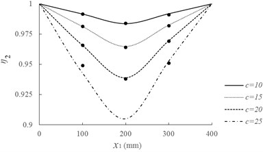
b) Reduction coefficient for 2nd natural frequency ( $η_{2}$ )

As can be seen from Fig. 4, $η_{1}$ and $η_{2}$ decrease with the increasing of crack width for simply supported beam with the same crack location. It indicates that the bigger the crack depth is, the greater the frequency reduction is. As for the effect of crack location, $η_{1}$ and $η_{2}$ present different variations. For $η_{1}$ , the minimum value is at the mid-span ( $x_{1} =$ 400 mm) for simply supported beam with the same crack depth. For $η_{2}$ , the minimum value is at the 1/4 span ( $x_{1} =$ 200 mm). The phenomena coincide with the change rules for 1st and 2nd mode shapes. The results are consistent with those obtained by Liang et al. [31], which can validate the effectiveness of the proposed method for dynamic analysis of simply supported cracked beam without vehicle.

5.1.2. Intact simply supported beam with vehicle

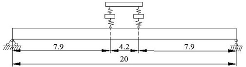
Two numerical examples are used to verify the accuracy of proposed method for simply supported beam with vehicles through the comparison of results calculated by proposed method and FEM (shown in Fig. 5).

Fig. 5Simply supported beam with vehicle (unit: m)

a) Case 1: Simply supported beam with single vehicle

b) Case 2: Simply supported beam with two vehicles

For finite element model, the beam is divided into 40 beam elements with length 0.5 m and each element has two nodes, in which each node has rotational and vertical displacements. The mass matrix $M$ and stiffness matrix $K$ of beam elements are formed using Lagrange interpolation function, and equation of vibration is derived as follows:

58

M_{b} \ddot{q} + K_{b} q = Φ^{T} F_{b},

where $M_{b} = Φ^{T} M Φ$ , $K_{b} = Φ^{T} K Φ$ , $\ddot{q}$ is the 2nd order derivation of modal coordinates for beam, $Φ$ is the first $n$ th order mode shape matrix of free vibration for beam, $F_{b}$ is the beam-vehicle interaction force:

59

F_{b} = H \{\begin{array}{l} P_{1} \\ P_{2} \end{array}\},

here, $H$ is the location matrix of external force point; $P_{1}$ and $P_{2}$ are the forces of front and back wheel on the beam, respectively.

Eq. (59) is substituted into Eq. (58). Equation of beam-vehicle system can be obtained combining with Eqs. (6-7), which is shown as follows [32]:

60

[\begin{matrix} M_{b} & 0 \\ 0 & M_{v} \end{matrix}] \{\begin{array}{l} \ddot{q} \\ {\ddot{u}}_{b} \end{array}\} + [\begin{matrix} K_{b} & K_{b v} \\ K_{b v}^{T} & K_{v} \end{matrix}] = 0,

where $M_{v}$ and $K_{v}$ are the mass and stiffness matrices of vehicle, respectively. $K_{b v}$ is coupling stiffness matrix of the beam-vehicle interaction system. Based on the finite element program constructed using MATLAB, modal properties of beam-vehicle system can be obtained by solving Eq. (60).

For the parameters of vehicle model, wheel masses $m_{t 1} = m_{t 2} =$ 1500 kg, sprung mass $m_{b} =$ 1.77×10⁴ kg, rotatory mass $I_{b} =$ 2.4×10⁵ kg·m², suspension spring constants $k_{t 1} = k_{t 2} =$ 3.0×10⁶ N/m, tire stiffness coefficients $k_{a 1} = k_{a 2} =$ 4.4×10⁶N/m, wheel distance $a =$ 4.2 m and $s_{1} = s_{2} =$ 0.5. The parameters of the beam are: length $L =$ 20 m, moment of inertia $I =$ 0.0647 m⁴, Young’s modulus $E =$ 3.0×10¹⁰Pa, mass per unit length $m =$ 948 kg.

The first three natural frequencies for cases 1 and 2 are calculated by the proposed method and FEM, respectively. The results are listed in Tables 1-2.

Table 1Calculation results of natural frequencies for case 1

Methods	1st	2nd	3rd
Present (rad/s)	38.4155	142.7383	318.2813
FEM (rad/s)	38.3898	142.6731	317.6233
Relative error (%)	0.0671	0.0457	0.2067

Table 2Calculation results of natural frequencies for case 2

Methods	1st	2nd	3rd
Present (rad/s)	38.8867	145.9531	319.2813
FEM (rad/s)	38.8237	145.9751	318.8869
Relative error (%)	0.1619	-0.0150	0.1235

As can be seen from the calculation results, relative errors for the first three natural frequencies for cases 1 and 2 are lower than 0.21 %. It reveals that the proposed method possesses favorable accuracy for vibration analysis of simply supported beams with vehicle.

5.2. Numerical simulation for simply supported multi-girder bridge

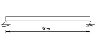
5.2.1. Simply supported bridge model

A simply supported bridge with uniform cross-section and 30 m span is adopted for numerical simulation and the bridge is composed of 4 girders (shown in Fig. 6(a)). According to the equivalent principle listed in section 2.1, cross section for this model can be simplified as a rectangular with width 0.8 m, height 1.5 m (shown in Fig. 6(b)). Elastic modulus is 3×10¹⁰ Pa, material density is 2500 kg/m³. The first three natural frequencies are calculated by the proposed method and listed in Table 3.

Fig. 6Simply supported bridge for numerical simulation (unit: m)

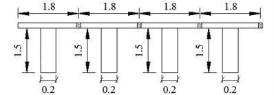
a) Sketch of cross section for simply supported bridge

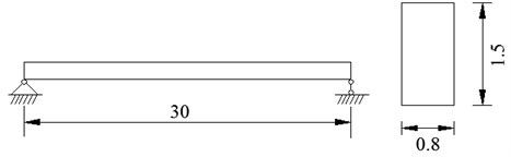
b) Simply supported bridge model and cross section

Table 3Natural frequencies for simply supported bridge without vehicle

$ω_{0}$	1st	2nd	3rd
Frequencies (rad/s)	16.4493	65.7974	148.0441

5.2.2. Cracked simply supported bridge without vehicle

Cracked simply supported bridge without vehicle is shown in Fig. 7. Its cross section is consistent with Fig. 6(b) and crack locations are 2, 4, …, 28 m from the left end of bridge, respectively. In order to demonstrate the effects of crack depth, crack position and crack number on natural frequencies of cracked simply supported bridge without vehicle, change ratio of natural frequencies considering cracks ( ${∆ ω}_{c}$ ) is used, which can be calculated by:

61

Δ ω_{c} = \frac{ω_{c} - ω_{0}}{ω_{0}} \times 100 %,

where $ω_{c}$ and $ω_{0}$ are natural frequencies calculated by the proposed method for cracked and intact simply supported bridge without vehicle, respectively.

Fig. 7Cracked simply supported bridge without vehicle

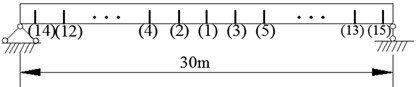
In order to demonstrate the effect of crack depth, the case of crack at position (1) (mid-span) with ratio of crack depth ( $c$ ) to cross section height ( $h$ ) ( $c / h$ ) varying from 10 % to 70 % (shown in Fig. 7) is adopted. The first three natural frequencies of bridge are calculated by the proposed method. Corresponding results are shown in Fig. 8.

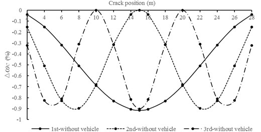
In order to demonstrate the effect of crack position, the cases of crack with $c / h =$ 15 % located at 2 m, 4 m, …, 26 m, 28 m from the left end of the bridge are used, respectively. Corresponding results are shown in Fig. 9.

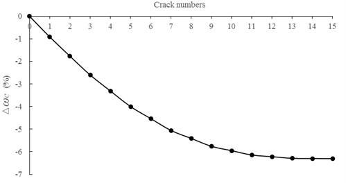
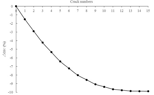
As for the effect of crack number, $c / h =$ 15 %, number of crack is 1 to 15, respectively. The results are shown in Fig. 10.

As can be seen from Fig. 8, ${∆ ω}_{c}$ of the first and third frequencies decrease nonlinearly with the increasing of crack depth. The greater crack depth is, the larger ${∆ ω}_{c}$ presents. However, crack depth has little influence on the second order frequency because crack is located at zero point for this mode.

In Fig. 9, ${∆ ω}_{c}$ is the largest if crack position is closer to the antinodal points of corresponding mode shape. Meanwhile, when the crack is located at the zero point of a certain mode, ${∆ ω}_{c}$ of corresponding frequencies are close to zero, which indicates that the crack has little influence.

Fig. 8Relationships between ∆ωc and crack depths for the first three natural frequencies

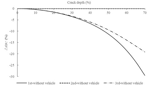
Fig. 9Relationships between ∆ωc and crack positions for the first three natural frequencies

In Fig. 10, ${∆ ω}_{c}$ decreases with the increasing of crack number. It indicates that the variation in frequency becomes larger as the number of crack increases and the influence of crack number on frequency is obvious.

Fig. 10Relationships between ∆ωc and crack numbers for the first natural frequency

5.2.3. Cracked simply supported bridge with one vehicle

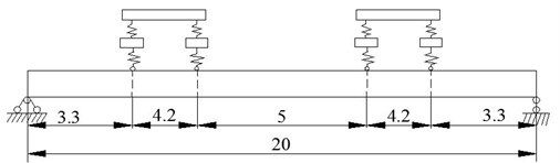
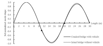
Cracked simply supported bridge with one vehicle is shown in Fig. 11, in which cross section is consistent with Fig. 6(b). For the parameters of vehicle model, wheel masses $m_{t 1} = m_{t 2} =$ 1500 kg, sprung mass $m_{b} =$ 1.7735×10⁴kg, rotatory mass $I_{b} =$ 2.4×10⁵kg·m², suspension spring constants $k_{t 1} = k_{t 2} =$ 2.0×10⁶N/m, tire stiffness coefficients $k_{a 1} = k_{a 2} =$ 1.4×10⁶N/m, wheel distance $a =$ 4.2 m and $s_{1} = s_{2} =$ 0.5. Crack positions are shown in Fig. 11, and crack depth is the same, $c / h =$ 30 %. The first three natural frequencies for intact bridge without vehicle and cracked bridge with vehicle are calculated by the proposed method and listed in Table 4. Corresponding normalized modal shapes are shown in Fig. 12.

Fig. 11Cracked simply supported bridge with single vehicle (unit: m)

As can be seen from Fig. 12, mode shapes of cracked bridge have significant changes at the crack positions, which is because the slopes of mode shapes at crack positions are discontinuous. Mode shapes calculated by the proposed method are coincident with the factual data, and it can be used for damage detection of bridge.

Table 4The first three natural frequencies for intact bridge without vehicle and cracked bridge with vehicle

Case	1st	2nd	3rd
Intact bridge without vehicle (rad/s)	16.4493	65.7974	148.0441
Cracked bridge with vehicle (rad/s)	17.0996	62.9297	147.7051

Fig. 12The first three normalized mode shapes (▲: crack position)

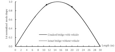
a) 1st normalized mode shape

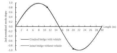
b) 2nd normalized mode shape

c) 3rd normalized mode shape

5.2.4. Simply supported bridge with one vehicle at different positions

Different vehicle parameters are determined and listed in Table 5. For these vehicles, each has four freedoms. Therefore, four natural frequencies ( $ω_{v v}^{1}$ , $ω_{v v}^{2}$ , $ω_{v v}^{3}$ and $ω_{v v}^{4}$ ) can be calculated for each vehicle model. Calculation results of natural frequencies for vehicles are listed in Table 6.

Table 5Four different vehicle parameters

Vehicle parameters	$m_{t 1}$ ( $m_{t 2}$ ) (kg)	$m_{b}$ (kg)	$I_{b}$ (kg·m²)	$k_{t 1}$ ( $k_{t 2}$ ) (N/m)	$k_{a 1}$ ( $k_{a 2}$ ) (N/m)	$a$ (m)	$s_{1}$ ( $s_{2}$ )
Vehicle 1	1500	17735	2.4×10⁵	2×10⁶	1.4×10⁶	4.2	0.5
Vehicle 2	1500	17735	2.4×10⁵	1×10⁶	0.6×10⁶	4.2	0.5
Vehicle 3	1500	17735	2.4×10⁵	0.2×10⁶	0.3×10⁶	4.2	0.5
Vehicle 4	1500	17735	2.4×10⁵	0.1×10⁶	0.4×10⁶	4.2	0.5

Table 6First four natural frequencies of vehicle models

Vehicle parameters	$ω_{v v}^{1}$ (rad/s)	$ω_{v v}^{2}$ (rad/s)	$ω_{v v}^{3}$ (rad/s)	$ω_{v v}^{4}$ (rad/s)
Vehicle 1	5.48	9.50	47.83	48.32
Vehicle 2	3.70	6.42	32.79	33.06
Vehicle 3	2.08	3.57	18.44	18.83
Vehicle 4	1.68	2.85	18.58	19.24

As for bridge model, it is consistent with Fig. 6(b) (shown in Fig. 13). The first natural frequencies are calculated by the proposed method for cases that the centerline of vehicle moves from support A to B (shown in Fig. 13). Change ratio of the first natural frequency considering vehicle ( ${∆ ω}_{v}^{1}$ ) is used to demonstrate the effect of vehicle, which can be calculated by:

62

Δ ω_{v}^{1} = \frac{ω_{V}^{1} - ω_{0}^{1}}{ω_{0}^{1}} \times 100 %,

where $ω_{v}^{1}$ is the first natural frequency of simply supported bridge with one vehicle calculated by the proposed method, $ω_{0}^{1}$ is the first natural frequency of intact bridge without vehicle calculated by the proposed method.

Results of ${∆ ω}_{v}^{1}$ for vehicle moving from A to B are shown in Fig. 14.

Fig. 13Simply supported bridge under one vehicle

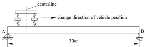
Fig. 14Relationship between ∆ωv1 and position of vehicle centerline

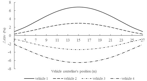
As can be seen from Fig. 14, ${∆ ω}_{v}^{1} > 0$ , when vehicle 1 or 2 is used. It indicates that the first natural frequency of simply supported bridge under vehicle 1 or 2 is higher than that without vehicle. However, ${∆ ω}_{v}^{1} < 0$ , when vehicle 3 or 4 is adopted. For all vehicle parameters, $ω_{0}^{1} =$ 16.4493 rad/s, which is between $ω_{v v}^{2}$ and $ω_{v v}^{3}$ . When parameters of vehicle 1 or 2 is adopted, $(ω_{0}^{1} - ω_{v v}^{2}) < (ω_{v v}^{3} - ω_{0}^{1})$ ; while $(ω_{0}^{1} - ω_{v v}^{2}) > (ω_{v v}^{3} - ω_{0}^{1})$ for vehicle 3 or 4. Based on above analysis, one conclusion can be obtained for assessing relative size of $ω_{0}^{1}$ and $ω_{V}^{1}$ . The closest vehicle frequency ( $ω_{v v}^{i}$ ) with $ω_{0}^{1}$ should be determined firstly. Then, $ω_{v v}^{i}$ and $ω_{0}^{1}$ are compared. If $ω_{v v}^{i} > ω_{0}^{1}$ , $ω_{V}^{1} < ω_{0}^{1}$ ; if $ω_{v v}^{i} < ω_{0}^{1}$ , $ω_{V}^{1} > ω_{0}^{1}$ . Other cases are also simulated to verify above results and that is effective. Moreover, the influence of vehicle on natural frequency decreases with the increasing of distance between the vehicle centerline and mid-span.

5.2.5. Cracked simply supported bridge with one vehicle at different positions

Model for cracked simply supported bridge with one vehicle at different positions is shown in Fig. 15. The first natural frequencies are calculated for cracked simply supported bridge with one vehicle in which the crack is located at mid-span and centerline of vehicle moves from A to B. In order to demonstrate the effect of bridge-vehicle interaction, change ratio of natural frequency considering crack and vehicle ( ${∆ ω}_{c v}^{1}$ ) is calculated by:

63

Δ ω_{c v}^{1} = \frac{ω_{c v}^{1} - ω_{0}^{1}}{ω_{0}^{1}} \times 100 %,

where $ω_{c v}^{1}$ is the first natural frequency of cracked simply supported bridge with one vehicle calculated by the proposed method.

In this paper, vehicle 1 and vehicle 3 (as listed in Table 6) are used, while crack depths ( $c / h$ ) are 0 %, 15 %, 20 %, 25 %. ${∆ ω}_{c v}^{1}$ for 8 cases are calculated and shown in Fig. 16.

In Fig. 16, coupled effects of vehicle and crack are presented for ${∆ ω}_{c v}^{1}$ of simply supported bridge. Increasing of crack depth leads to the reduction of ${∆ ω}_{c v}^{1}$ regardless of vehicle 1 or 3. If vehicle 3 is used, ${∆ ω}_{c}^{1} < 0$ , ${∆ ω}_{v}^{1} < 0$ and ${∆ ω}_{c v}^{1} < 0$ . If vehicle 1 is adopted, ${∆ ω}_{c}^{1} < 0$ , ${∆ ω}_{v}^{1} > 0$ and ${∆ ω}_{c v}^{1}$ ( $>$ or $<$ ) 0. As can be seen from Fig. 16, there are specific points for ${∆ ω}_{c v}^{1} = 0$ when crack depth $c / h =$ 15 %, 20 % and 25 %, respectively. Therefore, vehicle effect must be considered for crack identification of bridge.

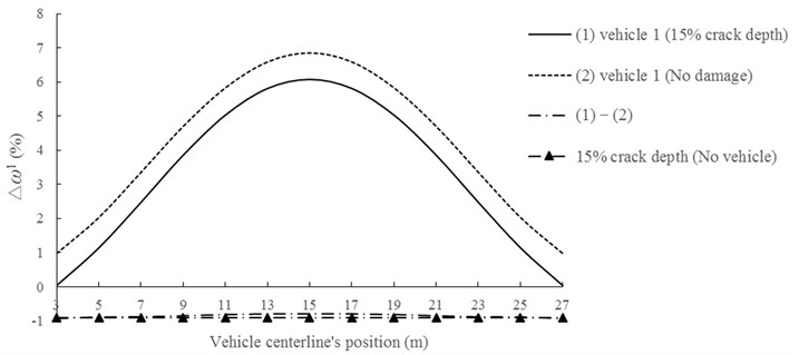
In order to demonstrate the effect of vehicle on crack identification, change ratio of the first natural frequency ( ${∆ ω}^{1}$ ) for simply supported bridge under vehicle 1 at mid-span, under vehicle 1 and with crack depth $c / h =$ 15 % at mid-span, only with crack depth $c / h =$ 15 % at mid-span are calculated by the proposed method, respectively. Corresponding results are shown in Fig. 17.

As shown in Fig. 17, difference of ${∆ ω}^{1}$ caused by (1) and (2) ((1)-(2)) is equal to that of 15 % crack depth without vehicle. Therefore, bridge-vehicle vibration system can be considered as a linear one, and crack-induced ${∆ ω}^{1}$ is comparable for bridge identification under the same parameters of vehicle.

Fig. 15Simply supported bridge with crack and vehicle

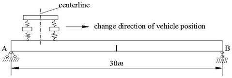
Fig. 16∆ωcv1 under different vehicle parameters and crack depths

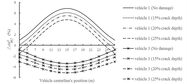
Fig. 17Change ratio of the first natural frequency due to bridge-vehicle interaction.

5.3. Numerical simulation for simply supported box-girder bridge

5.3.1. Simply supported box-girder bridge model

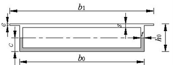
In order to verify the applicability of proposed method in integral bridge, a practical simply supported box-girder bridge is used for discussion. Geometrical parameters for this bridge are (shown in Fig. 18): $L =$ 30 m, $b_{0} =$ 6.5 m, $b_{1} =$ 7.5 m, $h_{0} =$ 1.5 m, $t =$ 0.18 m, $s =$ 0.20 m, $e =$ 0.08 m, and $c$ denotes the penetration depth of a sectional crack. The material parameters are: $E =$ 3×10¹⁰Pa, $ρ =$ 2500 kg/m³. The first three natural frequencies are calculated by the proposed method and listed in Table 7.

Fig. 18Simply supported box-girder bridge: a) longitudinal section; b) cross section

a)

b)

Table 7Natural frequencies for simply supported box-girder bridge without vehicle

$ω_{0}$	1st	2nd	3rd
Frequencies (rad/s)	23.5925	94.3699	212.3323

The local flexibility $θ$ due to a sectional crack can be calculated according to reference [33]. For a shallow open crack, the penetration depth ‘ $c$ ’ is contained within the bottom solid-sectional region [0 $\leq c \leq s$ ]:

64

θ = \frac{6 π r_{b} h_{0}}{[r_{b} - (r_{b} - 2 r_{t}) (1 - 2 r_{s})^{3}]} \int_{0}^{c / h_{0}} x F^{2} d x .

For a deeper open crack, depth ‘ $c$ ’ goes into the middle hollow-sectional region [ $s \leq c \leq (h_{0} - s)$ ]:

65

θ = \frac{6 π h_{0}}{[r_{b} - (r_{b} - 2 r_{t}) (1 - 2 r_{s})^{3}]} [r_{b} \int_{0}^{r_{s}} x F^{2} d x + 2 r_{t} \int_{r_{s}}^{c / h_{0}} x F^{2} d x],

where $r_{b} = b_{0} / h_{0}$ , $r_{t} = t / h_{0}$ , $r_{s} = s / h_{0}$ , and $F$ is a function of the relative depth $x$ :

66

F = \frac{\sqrt{2 / π x t a n π x / 2} [0.923 + 0.199 (1 - s i n π x / 2)^{4}]}{c o s π x / 2} .

Substituting the local flexibility coefficient ‘ $θ$ ’ into Eq. (10), transfer matrix can be calculated by the proposed method in this paper. Therefore, natural frequency and modal shape can be further obtained.

5.3.2. Cracked simply supported box-girder bridge without vehicle

Cases of various crack depths, positions and numbers are studied. Changes of crack depths, positions and numbers are the same as Section 5.2.2 and the results of ${∆ ω}_{c}$ are shown in Figs. 19-21.

As can be seen from Figs. 19-21, relationships between ${∆ ω}_{c}$ and crack depths, positions, numbers are similar with the conclusions obtained in Section 5.2.2. It reveals that the proposed method is general for different bridge type. For ${∆ ω}_{c}$ in Fig. 19, mutation point can be found due to crack going into the middle hollow-sectional region.

Fig. 19Relationship between ∆ωc and crack depth for box-girder bridge

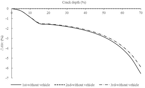
Fig. 20Relationship between ∆ωc and crack position for box-girder bridge

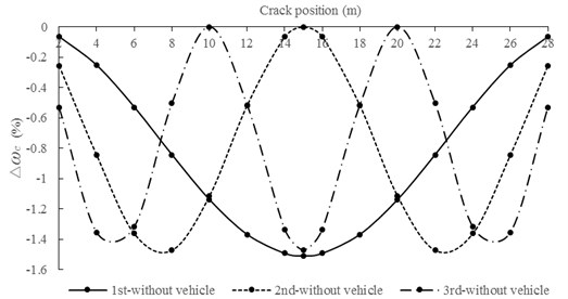
Fig. 21Relationship between ∆ωc and crack numbers for box-girder bridge

5.3.3. Cracked simply supported box-girder bridge with one vehicle

The parameters of vehicle are the same with Section 5.1.2. The depths of cracks are 30 %. Layouts of vehicle and cracks are shown in Figs. 22-23. The first three natural frequencies calculated by the proposed method are listed in Table 8, and normalized modal shapes are shown in Fig. 24.

Table 8Natural frequencies for box-girder bridge with and without vehicle

$ω$ (rad/s)	1st	2nd	3rd
Intact bridge without vehicle	23.5925	94.3699	212.3323
Cracked bridge without vehicle	22.9241	92.1462	211.9678
Intact bridge with vehicle	24.4643	94.4995	212.4756
Cracked bridge with vehicle	23.8520	92.2852	212.0898

Fig. 22Intact box-girder bridge with vehicle (unit: m)

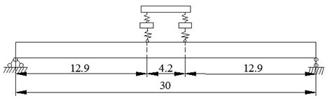
Fig. 23Cracked box-girder bridge with vehicle (unit: m)

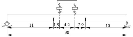
Fig. 24The first three order normalized mode shapes (▲: crack position)

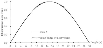
a) 1st normalized mode shape

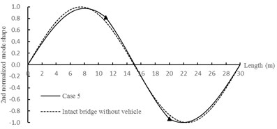
b) 2nd normalized mode shape

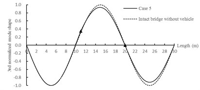
c) 3rd normalized mode shape

As shown in Fig. 24, the variation laws of normalized mode shapes are similar to that in Section 5.2.3 and there are also significant changes at crack positions.

5.3.4. Diagnosis of crack for a cracked simply supported box-girder with one vehicle

As discussed above, presence of cracks changes the characteristic equation and has influences on mode shapes and natural frequencies of the beam. In an inverse problem, crack positions and depths are unknown parameters, however, natural frequencies and mode shapes of damaged beam could be obtained through various testing techniques, and the 1st natural frequency and corresponding normalized mode shape can easily be determined experimentally. Because no experiment is carried out in this paper, a numerical example shown in Fig. 25 is used to identify the crack positions and depths. The 1st natural frequency ‘ $ω_{1}$ ’ and corresponding normalized mode shape ‘ $D_{1}$ ’ in Section 5.3.3 are adopted as input data for crack identification. $ω_{i n p u t} = ω_{1}$ , $D_{i n p u t} = D_{1} (1 + α σ \times r a n d n)$ . $r a n d n$ is the random generator function in MATLAB with a zero mean and a standard deviation of $σ$ , $α$ is error lever.

According to the matrix equation of all undetermined coefficients in Eq. (53), $p = s =$ 1, one can obtain the assembly matrix [ $H$ ] with dimension of 16×16. The undetermined coefficients correspond to $b_{1}^{1}$ , $R_{1}$ , $b_{2}^{1}$ and vehicle, respectively. Finally, there are 16 equations and 16 undetermined coefficients. Assuming crack positions and depths are known and $A_{b_{1}}^{1}$ is a constant ‘ $c$ ’, other undetermined coefficients could be solved by using any other fifteen equations. The undetermined coefficients of $b_{1}^{2}$ and $b_{2}^{2}$ are obtained by Eq. (21), the substitution of the undetermined coefficients and ‘ $ω_{i n p u t}$ ’ into Eq. (5) will determine the normalized mode shape of the bridge ‘ $d$ ’. The iterative algorithm is used to obtain the crack positions and depths by comparing normalized ‘ $D_{i n p u t}$ ’ and ‘ $d$ ’, and calculation process for this algorithm is as follows.

Fig. 25Simply supported box-girder bridge with vehicle and double cracks

(a) Assume initial values of crack positions ‘ $x$ ’ and depths ‘ $θ$ ’, which is a column vector with two elements respectively;

(b) According to ‘ $ω_{i n p u t}$ ’, ‘ $x$ ’ and ‘ $θ$ ’, the normalized mode shape ‘ $d$ ’ can be obtained, $∆ d = D_{i n p u t} - d$ , note that all normalized mode shapes ‘ $D_{i n p u t}$ ’ and ‘ $d$ ’ are consist of $q$ fixed position points;

(c) Sensitivity matrix $[S]$ can be calculated by Perturbation method [34]:

67

[S] = [\begin{array}{l} \frac{\partial d_{1}}{\partial x_{1}} & \frac{\partial d_{1}}{\partial x_{2}} & \frac{\partial d_{1}}{\partial θ_{1}} & \frac{\partial d_{1}}{\partial θ_{2}} \\ \frac{\partial d_{2}}{\partial x_{1}} & \frac{\partial d_{2}}{\partial x_{2}} & \frac{\partial d_{2}}{\partial θ_{1}} & \frac{\partial d_{2}}{\partial θ_{2}} \\ ⋮ & ⋮ & ⋮ & ⋮ \\ \frac{\partial d_{q}}{\partial x_{1}} & \frac{\partial d_{q}}{\partial x_{2}} & \frac{\partial d_{q}}{\partial θ_{1}} & \frac{\partial d_{q}}{\partial θ_{2}} \end{array}],

where:

\frac{\partial d_{i}}{\partial x_{1}} = \frac{d_{i} (ω_{i n p u t}, x_{1} + ε, x_{2}, θ_{1}, θ_{2}) - d_{i} (ω_{i n p u t}, x_{1}, x_{2}, θ_{1}, θ_{2})}{ε},

\frac{\partial d_{i}}{\partial x_{2}} = \frac{d_{i} (ω_{i n p u t}, x_{1}, x_{2} + ε, θ_{1}, θ_{2}) - d_{i} (ω_{i n p u t}, x_{1}, x_{2}, θ_{1}, θ_{2})}{ε},

\frac{\partial d_{i}}{\partial θ_{1}} = \frac{d_{i} (ω_{i n p u t}, x_{1}, x_{2}, θ_{1} + ε, θ_{2}) - d_{i} (ω_{i n p u t}, x_{1}, x_{2}, θ_{1}, θ_{2})}{ε},

\frac{\partial d_{i}}{\partial θ_{2}} = \frac{d_{i} (ω_{i n p u t}, x_{1}, x_{2}, θ_{1}, θ_{2} + ε) - d_{i} (ω_{i n p u t}, x_{1}, x_{2}, θ_{1}, θ_{2})}{ε}, |ε| ≪ 1, i = 1,2, \dots, q .

(d) Solve the residuals $Δ x$ and $Δ θ$ :

68

\{\begin{array}{l} Δ x \\ Δ θ \end{array}\} = [S]^{+} \cdot Δ d,

where $[S]^{+}$ is the generalized inverse matrix of $[S]$ using singular value decomposition.

$[S] = [U] [\begin{array}{l} Σ & 0 \\ 0 & 0 \end{array}] [V]^{H}$ , $[U]$ and $[V]$ are unitary matrices, $Σ = d i a g (σ_{1}, σ_{2}, \dots, σ_{r})$ , $σ_{i}$ is singular value of $[S]$ , $σ_{i} > 0$ , $r = r a n k ([S])$ . So $[S]^{+} = [V] [\begin{matrix} Σ^{- 1} & 0 \\ 0 & 0 \end{matrix}] [U]^{H}$ .

(e) Update the crack parameters:

69

x_{n e w} = x_{o l d} + p \cdot Δ x, θ_{n e w} = θ_{o l d} + p \cdot Δ θ,

where $p$ is an underrelaxation parameter and can be used to avoid overshoots and increase reliability of the algorithm in early steps of iterations.

(f) Iterate the procedures (b)-(e) until the residuals of $Δ x$ and $Δ θ$ become sufficiently small and satisfactorily.

The actual and predicted crack parameters calculated from the proposed identification algorithm are listed in Table 9.

Table 9Crack identification of a simply supported bridge with vehicle and double cracks

$α$	Crack parameters	Actual	Initial value	Predicted	Relative error (%)
0 %	Crack position (m)	11.00	9.00	10.967	–0.30
	Crack position (m)	20.00	23.00	20.090	0.45
	Crack depth (%)	30.00	20.00	30.117	0.39
	Crack depth (%)	30.00	20.00	29.877	–0.41
5 %	Crack position (m)	11.00	9.00	10.769	–2.10
	Crack position (m)	20.00	23.00	20.380	1.90
	Crack depth (%)	30.00	20.00	29.070	–3.10
	Crack depth (%)	30.00	20.00	31.140	3.80
10 %	Crack position (m)	11.00	9.00	11.473	4.3
	Crack position (m)	20.00	23.00	19.160	–4.2
	Crack depth (%)	30.00	20.00	28.470	–5.1
	Crack depth (%)	30.00	20.00	28.530	–4.9

From Table 9, the maximum relative error for crack position identification is 0.45 %, and it is 0.41 % for crack depth identification when $α =$ 0 %. Relative error increases with increasing of $α$ , and it is within 5.5 % for both position and depth identifications when $α =$ 10 %. The results reveal that the proposed algorithm for crack identification possesses favorable accuracy and robustness to noise.

6. Conclusions

In this paper, free vibration analysis of cracked simply supported bridge under arbitrary number of vehicles is presented. The exact solutions for natural frequencies and mode shapes of cracked bridge considering bridge-vehicle interaction are derived based on Euler-Bernoulli beam theory and numerical assembly method. Numerical simulation on simply supported bridge is used to verify its feasibility. Following conclusions can be obtained:

1) The first two natural frequencies of simply supported bridge with different crack depths are calculated by the proposed method. Reduction coefficients for natural frequencies are consistent with the present study. The first three natural frequencies of simply supported bridge under one and two vehicles are analyzed, respectively. The results are in good agreement with FEM. It reveals that the proposed method possesses favorable reliability.

2) Simply supported multi-girder bridge is adopted and simplified. Change ratio of natural frequencies considering cracks ( ${∆ ω}_{c}$ ) is presented to investigate the influences of crack depth, position and number, respectively. For crack depth, the greater depth is, the larger ${∆ ω}_{c}$ presents for the first and third frequencies. However, it has little influence on the second order frequency. For crack position, ${∆ ω}_{c}$ is the largest if crack position is closer to the antinodal points of corresponding mode shape. For crack numbers, ${∆ ω}_{c}$ decreases with the increasing of crack number. Moreover, significant changes of modal shapes occur at the crack positions.

3) The influences of vehicle parameters on modal properties are also investigated. For intact bridge under one vehicle with four different parameters, the first natural frequencies present different change rules, which are closely associated with vehicles parameters. Corresponding judgment method is also proposed based on frequencies of vehicle and bridge without vehicle. Moreover, the influence of vehicle on natural frequency decreases with the increasing of distance between the vehicle centerline and mid-span. For cracked simply supported bridge with one vehicle at different positions, coupled effects of vehicle and crack are presented for frequency changes, and vehicle effect must be considered for crack identification of bridge. Meanwhile, bridge-vehicle vibration system can be considered as a linear one, and crack-induced frequency changes are comparable for bridge identification under the same parameters of vehicle.

4) The proposed method is applicable for simply supported box-girder bridge. An effective approach for crack identification is proposed, which presents favorable accuracy.

References

Kim C. Y., Jung D. S., Kim N. S., Kwon S. D., Feng M. Q. Effect of vehicle weight on natural frequencies of bridges measured from traffic-induced vibration. Earthquake Engineering and Engineering Vibration, Vol. 2, Issue 1, 2003, p. 109-115.

Publisher
Fu C. Dynamic behavior of a simply supported bridge with a switching crack subjected to seismic excitations and moving trains. Engineering Structures, Vol. 110, 2016, p. 59-69.

Publisher
Dimarogonas A. D. Vibration of cracked structures: a state of the art review. Engineering Fracture Mechanics, Vol. 55, 1996, p. 831-57.

Publisher
Haisty B. S., Springer W. T. A general beam element for use in damage assessment of complex structures. Journal of Vibration and Acoustics, Vol. 110, Issue 3, 1988, p. 389-394.

Publisher
Narkis Y. Identification of crack location in vibrating simply supported beams. Journal of Sound and Vibration, Vol. 172, Issue 4, 1994, p. 549-558.

Publisher
Christides S., Barr A. D. S. One dimensional theory of cracked Bernoulli-Euler beams. International Journal of Mechanical Sciences, Vol. 26, Issues 11-12, 1984, p. 639-648.

Publisher
Chondros T. G., Dimarogonas A. D., Yao J. A continuous cracked beam vibration theory. Journal of Sound and Vibration, Vol. 215, Issue 1, 1998, p. 17-34.

Publisher
Yang F., Swamidas A. S. J., Seshadri R. Crack identification in vibrating beams using the energy method. Journal of Sound and Vibration, Vol. 244, Issue 2, 2001, p. 339-357.

Publisher
Saavedra P. N., Cuitino L. A. Crack detection and vibration behavior of cracked beams. Computers and Structures, Vol. 79, Issue 16, 2001, p. 1451-1459.

Publisher
Pestel E. C., Leckie F. A. Matrix methods in elasto mechanics. Journal of Applied Mechanics, Vol. 31, 3, p. 1964-574.

Publisher
Ostachowicz W. M., Krawczuk M. Analysis of the effect of cracks on the natural frequencies of a cantilever beam. Journal of Sound and Vibration, Vol. 150, Issue 2, 1991, p. 191-201.

Publisher
Lin H. P., Chang S. C., Wu J. D. Beam vibrations with an arbitrary number of cracks. Journal of Sound and Vibration, Vol. 258, Issue 5, 2002, p. 987-999.

Publisher
Zibdeh H. S. Stochastic vibration of an elastic beam due to random moving loads and deterministic axial forces. Engineering Structures, Vol. 17, Issue 7, 1995, p. 530-535.

Publisher
Abu-Hilal M. Dynamic response of a double Bernoulli-Euler beam due to a moving constant load. Journal of Sound and Vibration, Vol. 297, Issues 3-5, 2006, p. 477-491.

Publisher
Liu X. W., Xie J., Wu C., Huang X. C. Semi-analytical solution of vehicle-bridge interaction on transient jump of wheel. Engineering Structures, Vol. 30, Issue 9, 2008, p. 2401-2412.

Publisher
Fryba L. A rough assessment of railway bridges for high speed trains. Engineering Structures, Vol. 23, Issue 5, 2001, p. 548-556.

Publisher
Yau J. D., Wu Y. S., Yang Y. B. Impact response of bridges with elastic bearings to moving loads. Journal of Sound and Vibration, Vol. 248, Issue 1, 2001, p. 9-30.

Publisher
Ichikawa M., Miyakawa Y., Matsuda A. Vibration analysis of the continuous beam subjected to a moving mass. Journal of Sound and Vibration, Vol. 230, Issue 3, 2000, p. 493-506.

Publisher
Rieker J. R., Trethewey M. W. Finite element analysis of an elastic beam structure subjected to a moving distributed mass train. Mechanical Systems and Signal Processing, Vol. 13, Issue 1, 1999, p. 31-51.

Publisher
Liu J. B., Du X. L. Dynamics of Structures. China Machine Press, Beijing, 2005.

Search CrossRef
Yang Y. B., Yau J. D. Vehicle-bridge interaction element for dynamic analysis. Journal of Structural Engineering, Vol. 123, Issue 11, 1997, p. 1512-1518.

Publisher
Esmailzadeh E., Jalili N. Vehicle-passenger-structure interaction of uniform bridges traversed by moving vehicles. Journal of Sound and Vibration, Vol. 260, Issue 4, 2003, p. 611-635.

Publisher
Song M. K., Noh H. C., Choi C. K. A new three-dimensional finite element analysis model of high-speed train-bridge interactions. Engineering Structures, Vol. 25, Issue 13, 2003, p. 1611-1626.

Publisher
Nasrellah H. A., Manohar C. S. A particle filtering approach for structural system identification in vehicle-structure interaction problems. Journal of Sound and Vibration, Vol. 329, Issue 9, 2010, p. 1289-1309.

Publisher
Zhang N., Xia H. Dynamic analysis of coupled vehicle-bridge system based on inter-system iteration method. Computers and Structures, Vol. 114, Issue 115, 2013, p. 26-34.

Publisher
Yang Y. B., Lin C. W. Vehicle-bridge interaction dynamics and potential applications. Journal of Sound and Vibration, Vol. 284, Issue 1, 2005, p. 205-226.

Publisher
Bilello C., Bergman L. A. Vibration of damaged beams under a moving mass: theory and experimental validation. Journal of Sound and Vibration, Vol. 274, Issues 3-5, 2004, p. 567-582.

Publisher
Lin H. P., Chang S. C. Forced responses of cracked cantilever beams subjected to a concentrated moving load. International Journal of Mechanical Sciences, Vol. 48, Issue 12, 2006, p. 1456-1463.

Publisher
Yoon H. I., Son I. S. Dynamic behavior of cracked pipe conveying fluid with moving mass based on Timoshenko beam theory. Journal of Mechanical Science and Technology, Vol. 18, Issue 12, 2004, p. 2216-2224.

Publisher
Li Q. S. Free vibration analysis of non-uniform beams with an arbitrary number of cracks and concentrated masses. Journal of Sound and Vibration, Vol. 252, Issue 3, 2002, p. 509-525.

Publisher
Liang R. Y., Hu J., Choy F. Theoretical study of crack-induced eigenfrequency changes on beam structures. Journal of Engineering Mechanics, Vol. 118, Issue 2, 1992, p. 384-396.

Publisher
Law S. S., Zhu X. Q. Dynamic behavior of damaged concrete bridge structures under moving vehicular loads. Engineering Structures, Vol. 26, Issue 9, 2004, p. 1279-1293.

Publisher
Zheng D. Y., Fan S. C. Vibration and stability of cracked hollow-sectional beams. Journal of Sound and Vibration, Vol. 267, Issue 4, 2003, p. 933-954.

Publisher
Chen S. H. Matrix Perturbation Theory of Structure Vibration Analysis. Chongqing Press, Chongqing, 1991.

Search CrossRef

Cited by

An exact closed-form explicit solution of free transverse vibration for non-uniform multi-cracked beam

Shahram Hadian Jazi | Mostafa Hadian | Keivan Torabi

(2024)

Material Performance of Anti-Differential Disturbance Concrete Based on the Vehicle–Bridge Coupling Vibration Theory

Guosheng Zeng | Xuefei Shi | Jun Song | Chaoyu Zhu

(2023)

Damage detection for bridge structures under vehicle loads based on frequency decay induced by breathing cracks

Jinsong Zhu | Yifeng Zhang

(2023)

Transfer Matrix Method for Calculating the Transverse Load Distribution of Articulated Slab Bridges

Kaiqiang Guo | Zhao Liu | Jesús-Miguel Bairán

(2022)

Dynamic Response of a Nonuniform Timoshenko Beam with Elastic Supports, Subjected to a Moving Spring-Mass System

(2018)

Free Vibration Analysis of a Uniform Continuous Beam with an Arbitrary Number of Cracks and Spring-Mass Systems

Guojin Tan | Zhiqing Zhu | Wensheng Wang | Yongchun Cheng

(2018)

Direct and inverse problems on free vibration analysis of cracked non-uniform beams carrying spring-mass systems by finite element method

Guojin Tan | Ziyu Liu | Jinghui Shan | Chunli Wu

(2017)

About this article

Received

12 February 2016

Accepted

04 September 2016

Published

30 September 2016

SUBJECTS

Fault diagnosis based on vibration signal analysis

DOI

https://doi.org/10.21595/jve.2016.16908

Keywords

simply supported bridge

free vibration

crack

vehicle

transfer matrix method

Acknowledgements

The authors express their appreciation for financial supports of National Natural Science Foundation of China under Grants Nos. 51478203 and 51408258; China Postdoctoral Science Foundation funded Project (Nos. 2014M560237 and 2015T80305); Fundamental Research Funds for the Central Universities and Science (JCKYQKJC06), and Technology Development Program of Jilin Province.

This is an open access article distributed under the Creative Commons Attribution License, which permits unrestricted use, distribution, and reproduction in any medium, provided the original work is properly cited.

Previous article in issue Previous Next article in issue Next

Research article

2024 03 02

An analytical model for the analysis of vibration and energy flow in a clamped stiffened plate using integral transform technique

Hui Guo, Kai Zhang

Research article

2023 10 20

Assessment of cracks in beams using changes in the measured frequencies and Particle Swarm Optimization

Horea-Adrian Grebla, Vasile Catalin Rusu, Gilbert-Rainer Gillich, Thu Hang Bui

Research article

2020 06 29

Influence of bridge geometric nonlinearity on dynamic response of vehicle-bridge coupling system

Zhijun Ni, Liangliang Zhang, Tao Wu, Binbin Zhang, Teng Wang

Research article

2019 11 28

Free vibration analysis of simply supported rectangular plates

Ganesh Naik Guguloth, Baij Nath Singh, Vinayak Ranjan

G. Tan, W. Wang, and Y. Jiao, “Free vibration analysis of a cracked simply supported bridge considering bridge-vehicle interaction,” Journal of Vibroengineering, Vol. 18, No. 6, pp. 3608–3635, Sep. 2016, https://doi.org/10.21595/jve.2016.16908

Copy Extrica

Copied to clipboard!

TY  - JOUR
DO  - 10.21595/jve.2016.16908
UR  - https://doi.org/10.21595/jve.2016.16908
TI  - Free vibration analysis of a cracked simply supported bridge considering bridge-vehicle interaction
T2  - Journal of Vibroengineering
AU  - Jiao, Yubo
AU  - Tan, Guojin
AU  - Wang, Wensheng
PY  - 2016
DA  - 2016/09/30
PB  - JVE International Ltd.
SP  - 3608-3635
IS  - 6
VL  - 18
SN  - 1392-8716
ER  - 

Copy Ris

Copied to clipboard!

@article{Jiao_2016,
	doi = {10.21595/jve.2016.16908},
	url = {https://doi.org/10.21595/jve.2016.16908},
	year = 2016,
	month = {sep},
	publisher = {{JVE} International Ltd.},
	volume = {18},
	number = {6},
	pages = {3608--3635},
	author = {Yubo Jiao and Guojin Tan and Wensheng Wang},
	title = {Free vibration analysis of a cracked simply supported bridge considering bridge-vehicle interaction},
	journal = {Journal of Vibroengineering}
}

Copy Bibtex

Copied to clipboard!

[1]Y. Jiao, G. Tan, and W. Wang, “Free vibration analysis of a cracked simply supported bridge considering bridge-vehicle interaction,” Journal of Vibroengineering, vol. 18, no. 6, pp. 3608–3635, Sep. 2016, doi: 10.21595/jve.2016.16908.

Copy IEEE

Copied to clipboard!

Jiao, Yubo, Guojin Tan, and Wensheng Wang. “Free Vibration Analysis of a Cracked Simply Supported Bridge Considering Bridge-Vehicle Interaction.” Journal of Vibroengineering 18, no. 6 (September 30, 2016): 3608–35. https://doi.org/10.21595/jve.2016.16908.

Copy Chicago

Copied to clipboard!

Free vibration analysis of a cracked simply supported bridge considering bridge-vehicle interaction

Abstract

1. Introduction

2. Theoretical background

2.1. Simplified models for bridge and vehicle

2.2. Equation of motion and displacement function

2.2.1. Equation of motion and displacement function for bridge

2.2.2. Equation of motion and displacement function for vehicle

3. Equations of undetermined coefficients

3.1. Equations of bridge sections

3.2. Equations at wheels

3.3. Equations from motion of vehicles

3.4. Equations from boundary conditions

4. Determination of natural frequencies and modal shapes

5. Numerical simulation and discussions

5.1. Reliability of the proposed method

5.1.1. Cracked simply supported beam without vehicle

5.1.2. Intact simply supported beam with vehicle

5.2. Numerical simulation for simply supported multi-girder bridge

5.2.1. Simply supported bridge model

5.2.2. Cracked simply supported bridge without vehicle

5.2.3. Cracked simply supported bridge with one vehicle

5.2.4. Simply supported bridge with one vehicle at different positions

5.2.5. Cracked simply supported bridge with one vehicle at different positions

5.3. Numerical simulation for simply supported box-girder bridge

5.3.1. Simply supported box-girder bridge model

5.3.2. Cracked simply supported box-girder bridge without vehicle

5.3.3. Cracked simply supported box-girder bridge with one vehicle

5.3.4. Diagnosis of crack for a cracked simply supported box-girder with one vehicle

6. Conclusions

References

Cited by

About this article

Related Articles