Abstract
The performance of vehicle active safety electric control system often depends on accurate estimation of the tire/road friction coefficient. The control target parameters should change along with the tire/road friction coefficient and implement different control strategy and control algorithm. Due to the interaction mechanism between tire and ground is very complex, so the multi-freedom rim-beam dynamic model with tire dynamic friction model is set up in this paper. And the key parameters influence characteristics was simulated analysis and the tire/road coefficient estimation model was established. The wheel speed signal conditioning circuit was designed and filtered out the noise by soft threshold wavelet. Finally, vehicle field tests of high, low and joint road were carried out, and the brake pressure (brake torque), vehicle velocity (wheel speed), slip ratio and wheel speed sensor sine wave time-frequency analysis and tire-road friction coefficient estimation were analyzed.
1. Introduction
Vehicles movement stability on the road depends on the accurate control of tire/road forces. The road features real-time accurate identification can provide decision-making basis for the vehicle active safety device (such as ABS/EBD/TCS/ESP, ACC, etc.). At present, the road recognition methods mainly have sensor direct detection method (light, sound, microwave, image, etc.), vehicle dynamics and kinematics method and multi-sensor information fusion estimation method based on vehicle dynamics. Although the former method has good effect, but it needs expensive sensing test system and is difficult to achieve large-scale commercial applications. The two latter methods mainly are applied to vehicle braking condition and calculates the tire-road friction coefficient by the relationship curve between the brake factor and tire/road friction coefficient. But because of the complexity of the interaction between tire and road, especially the dynamic friction characteristics, the road friction coefficient real-time robust identification has great difficulty.
A Novel Wireless Piezoelectric Tire Sensor was used to Estimate the Tire-Road Friction Coefficient by the lateral carcass deformations from the radial and tangential deformations [1]. Shim Taehyun proposed a model based road friction estimation algorithm from easily measured signals such as yaw rate and wheel speed [2]. Changsun Ahn presented four methods to estimate the friction coefficient based on four different excitation conditions and these four methods were then integrated to increase the working range of the estimator and to improve robustness [3]. D. J. Lee presented a sliding-mode scheme to identify the system state and the parameter variation of a torsional tire system and the recursive least-squares method with a forgetting facto is used to estimate the parameter variations of the tire system and the tire–road friction force without a friction model using the information retrieved from the equivalent input for sliding motion [4]. Gurkan Erdogan studied the development and experimental evaluation of a novel redundant-wheel based adaptive feedforward vibration cancellation system for friction coefficient estimation [5]. Rajesh Rajamani proposed three different algorithms based on the types of sensors available – one that utilizes engine torque, brake torque, and GPS measurements; one that utilizes torque measurements and an accelerometer; and one that utilizes GPS measurements and an accelerometer [6]. Rongrong Wang proposed a tire cornering stiffness coefficient and TRFC estimation method based on the longitudinal tire force difference between the two sides of the vehicle [7]. Luis Alvarez designed an adaptive control scheme for emergency braking of vehicles based on a LuGre dynamic model for the tire-road friction [8].
2. The wheel/road dynamic characteristics
2.1. Rim-beam-road dynamic model
The relationship between the tire and road is surface contact under load. Considering tread rubber has quality and elasticity, we use the spring and mass system simulate the movement status of tread grounding area and is shown in Fig. 1, and the system dynamics equation is as follows:
where, is the rim inertia moment, is rim angular velocity (is also angular velocity of the wheel speed sensor measured and the measured waveform is presented in the third section of this article), is the rim angle, is braking torque (its characteristics was obtained by experiments, and descripted as Eq. (21) or Eq. (22)), and are sidewall’s torsional stiffness and damping coefficient, is tire ring inertia moment, ω2 is tire ring angular velocity, is tire ring angle. is the tire rolling radius. is tire longitudinal adhesion force, which can be obtained by tire LuGre dynamic friction model as Eq. (4).
The tire LuGre dynamic friction model can accurately describe the transient and steady-state characteristics of tires friction force, tire friction process Stribeck effect, friction slip effect and hysteresis effect [8]. The two friction contact faces are assumed as two rigid bodies, they contact each other by elastic mane. When applying tangential force on one any contact body along the contact surface, the “mane” will deflect like spring and the interface friction force will increase. If the friction force is enough, the mane has excessive deflection and slip, and we use the variable describe the “mane average elastic deflection”, the friction model is established and is shown in Fig. 1. Contact translation friction force is a function of relative speed, it can clearly describe the Stribeck effect, coulomb friction and viscous friction effect, and is shown in Fig. 2.
Fig. 1Hub/tire model with LuGre friction model
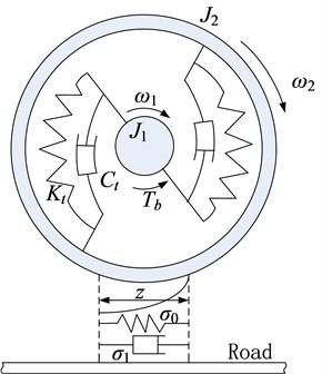
Fig. 2Stribeck effect of LuGre friction model
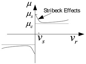
Assuming tire grounding mark as a stress point and regardless of tire pressure distribution change along the grounding mark, we only use the form of a simple time domain differential equation to describe the model. Lumped dynamic tire LuGre model can be represented as the following:
where is the longitudinal rubber lumped stiffness, is the damping coefficient of the longitudinal lumped rubber, is relative viscous damping coefficient, is the normalized coulomb friction, is normalized static friction force (), is the Stribeck relative velocity, is the tire vertical load, is the relative speed, is the internal friction state (which is only the state variable related to the time in lumped model), is the Stribeck effect index ([0.5,2]); is the road surface coefficient, the value of dry and wet asphalt pavement, snow and ice road is 1, 0.6, 0.2, 0.1 respectively.
Vertical force of each wheel ( respectively corresponding to the front left, front right, rear left and rear right, the following is similar) are obtained by following equations:
where is the vehicle longitudinal velocity, is lateral velocity, is yaw angular velocity, is body roll angle, is the vehicle mass center height from the ground; is vehicle wheel base; is ratio of the front axle roll stiffness in total roll stiffness; is the lateral acceleration, and , is roll angle acceleration; is the vehicle total quality; is the sprung mass; is the sprung load centroid distance from roll axis; is the centroid distance from front axle; is the centroid distance from rear axle; is the wheel track. All these state variables of the vehicle are obtained by in-situ test, and limited to space most of the measured waveforms are not presented in this paper.
At the same time, the vehicle longitudinal motion differential equation is as follows:
where, is the wind resistance, , is four wheels longitudinal force respectively. The vehicle basic parameters are shown in Table 1.
Table 1The basic parameters
Parameter | Value | Unit | Parameter | Value | Unit |
100 | 1/m | 0.32 | m | ||
0.7 | s/m | 1701 | kg | ||
0.011 | s/m | 0.12 | kg∙m2 | ||
15 | N∙m∙s/rad | 1.1 | kg∙m2 | ||
13000 | N∙m/rad | 0.005 | N∙s2/m | ||
0.35 | [-] | 9.8 | m/s2 | ||
0.5 | [-] | 0.5 | [-] | ||
10 | m/s |
2.2. Brake model
The vehicle front and rear brake are both disc brake, the braking torque is expressed as follows:
where a is contact area of brake caliper and disc; is the caliper number of a single wheel brake; is the friction coefficient between brake caliper and disc; is the effective friction radius; is the braking efficiency; is the wheel brake cylinder pressure. Considering the mechanical and hydraulic delay influence of the braking system, the braking system is simplified as a first-order lag system, and the braking torque was revised as follows:
where and are the time constants.
2.3. The model simulation
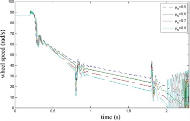
The vehicle velocity and wheel speed simulation results are shown in Fig. 3 on joint road (concrete road→ice road→concrete road, namely 1→0.1→1) under emergency braking with anti-lock braking system. It can be seen that the tire speed presents obvious dynamic characteristics at the braking torque implementation and joint road. the influence of Stribeck effect index on wheel speed simulation results is shown in Fig. 4, it can be seen that when 1.5 or 2, there has oscillation when velocity is low, that is value should not be too big. the influence of the longitudinal rubber lumped damping coefficient on wheel speed simulation result is shown in Fig. 5. It can be seen when has larger value, wheel speed has oscillation, so value should not be too big. the influence of normalized static friction on wheel speed simulation result is shown in Fig. 6, its impact is the same as and .
Fig. 3simulation results on joint road
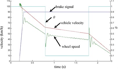
Fig. 4α influence on wheel speed
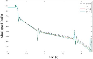
Fig. 5σ1 influence on wheel speed
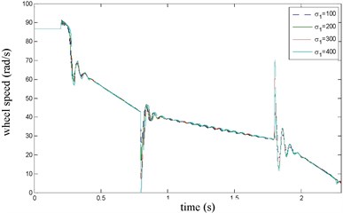
Fig. 6μs influence on wheel speed
2.4. Road friction coefficient estimation model
Assuming that the acceleration can be measured, road friction coefficient can be defined as . the state observer of state variables z can be deduced by the Eq. (4) as follows:
where is pavement parameters estimated value and there has the following estimation process:
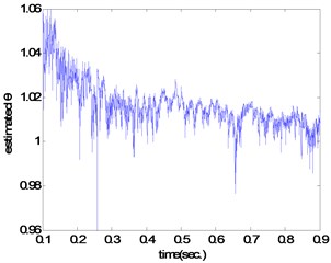
where is adjustment coefficient ). the estimated result of large friction coefficient road is shown in Fig. 7, and we can see that the estimated value is about equal to the real value (). Using tire dynamic friction model the estimation methods describe the change of the tire/road contact friction and various parameters have clear physical meaning, which can accurately describe the tire/road friction behavior. But in the actual process of estimation we need to analyze the stability of the observer and ensure enough robustness.
Fig. 7θ estimated result of large friction coefficient road (μ= 0.8)
3. Real vehicle experiment and analysis
3.1. Wheel speed signal conditioning circuit
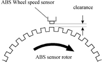
Wheel speed sensor adopts variable reluctance type, it consists of rotating gear and relatively static induction coil, it is shown in Fig. 8. When the gear turns near the induction coil, coil will produce AC voltage due to impedance periodical change, and the frequency of the AC voltage is proportional to the gear speed and the teeth number. in the case of gear teeth have been confirmed, sensing coil output voltage frequency is proportional to the speed of the gear. and magnetic resistance change speed has big effect on pulse voltage amplitude, the output voltage is high when magnetic resistance changes quickly, and the output voltage is low when magnetic resistance changes slowly. It is generally between dozens of millivolt to dozens of V.
Fig. 8Magnetoelectric wheel speed sensors
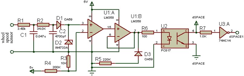
Wheel speed sensor signal conditioning circuit is shown in Fig. 9. Using passive second order RC filter, the passive filter cutoff frequency is , where is resistance, is capacitance. and according to the highest wheel speed, we take fc=1KHz. Impedance value is chosen freely, and we take 3.4 KΩ, 0.047 μF. According to the impedance distribution principle (rom low to high), 34 K Ω, 4700 pF in secondary RC filter circuit. D1 is OA59 germanium detector diode, it filters the filtered sine waveform negative half cycle, D2 is 5.1 V zener diode of IN4733 model.
The signal is converted to the rectangular wave signal with the same frequency by LM358 voltage comparator composed of U1:A and U1:B. the comparing voltage is 0.233 V, and when the input voltage is less than the , output is low, whereas the output is high. Signal is further filtered by the D3 and R5. R6 is flow limit resistance, U2 is light coupling isolator, its C and E side power are supplied by dSPACE (including U3:A power supply). Because there has “bent shoulders” during the square wave output from low level to high level, we smooth the signal and make it stable by rectangular wave through R7 and 74HC14 Schmitt trigger, and finally send it to dSPACE1 for wheel speed signal acquisition. in addition, in order to reduce and restrain the disturb by the voltage instability of controll circuit for the wheel speed sensor signal and the signal processing circuit, the required 5 V power supply system has a dedicated 7805 three-terminal voltage regulator integrated circuit which works from a 12 V, 1.25 A convert power source.
Fig. 9Wheel speed sensor signal conditioning circuit
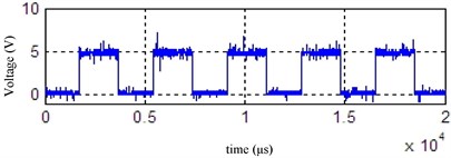
The adjusted rectangular wave is shown in Fig. 10, it can be seen the wheel speed sensor signal conditioning circuit is reasonable, it can satisfy the requirements of the wheel speed signal acquisition.
Fig. 10Wheel speed modulation circuit output signal
3.2. Test signal wavelet filter
The noise signal of real vehicle tests usually is high frequency white noise, so it's best to use wavelet decomposition method for noise elimination. Namely the signal is decomposed by wavelet firstly, and due to the noise signal contains high frequency detail largely, thus we can deal with the wavelet decomposition coefficients by the threshold, and then we implement the signal wavelet reconstruction. Among which the key is how to choose the threshold value and quantize the threshold, usually we adopt a given soft threshold denoising method and often use SNR (Signal to Noise Ratio) and MSE (mean square error) to evaluate denoising effect commonly.
where is the standard original signal, is processed estimated signal. Among them, it is better when the SNR is larger, but MSE as small as possible.
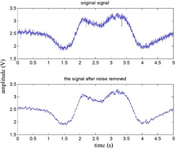
The brake pressure and lateral acceleration time domain before and after denoising waveform by given soft threshold denoising method are shown in Fig. 11 and Fig. 12 respectively. the SNR is 34.4622 and MSE is 1.28e-05 in Fig. 11. the SNR is 45.9048 and MSE is 1.64e-4 in Fig. 12. It can be seen waveform curve smoothing effect after denoising is better using a given soft threshold denoising method.
Fig. 11Brake pressure before and after denoising
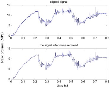
Fig. 12Lateral acceleration before and after denoising
3.3. Field experiment analysis
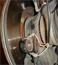
The brake caliper fixed arm will produce deformation during braking, and strain gauge was pasted on the brake arm up and down sides, which is shown in Fig. 13(a). and then we can get the relationship between strain voltage signal and the actual braking torque by torque calibration test. the front right wheel calibration formula between strain voltage and braking torque is as follows:
where is the braking torque, unit is N∙m; is the measured sum strain voltage of the brake caliper arm up and down sides, unit is V. the rear right wheel calibration formula between strain voltage and braking torque is as follows:
Because the structure of the coaxial left and right brake are exactly same and we only carried out the front right and rear right wheel torque calibration experiments, that we consider the wheel transfer characteristic of the left and right side wheel are same.
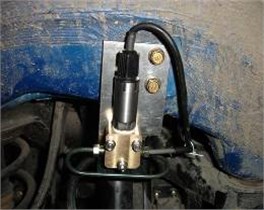
Furthermore, the transfer coefficient between brake pressure and brake torque can be obtained through the real vehicle experiment, four-wheel cylinder pressure was collected by four pressure sensors, and is shown in Fig. 13(b). Experimental method is as follows: we implemented straight braking at about 30 km/h on dry asphalt pavement. Sampling rate is 1000 Hz, sampling time is 10 s, and filter all data at 100Hz. According to the experimental results, we can get the transfer function between the front wheel brake pressure (MPa) and the brake torque (N∙m) as follows:
where is the gain coefficient, the unit is N∙m/MPa; is the system one-order inertial time constant, the unit is s.
For the rear wheel:
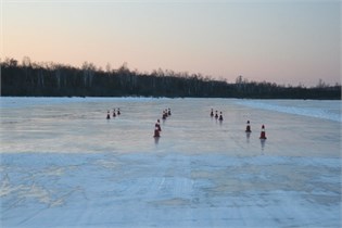
Finally, the real vehicle experiment has been carried out in a winter proving ground, the scene is shown in Fig. 13(c). We mainly collected vehicle brake pressure, wheel speed and vehicle body inertia and navigation parameters and estimated the road friction coefficient. All brake tests were carried out under straight line braking and ABS/ESP system worked normally.
Fig. 13Field experiments photos
a)
b)
c)
3.3.1. Dry concrete pavement experimental results
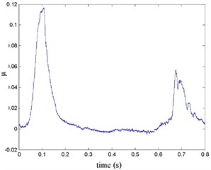
The front right and the rear right brake pressure are shown in Fig. 14 during emergency braking on the dry concrete pavement (friction coefficient 0.8), and their brake torque are shown in Fig. 15. FR wheel-speed sine waveform and its Wigner Ville distribution are shown in Fig. 16. RR wheel sine waveform and its Wigner Ville distribution are shown in Fig. 17. the vehicle velocity and wheel speed experimental results are shown in Fig. 18, road friction coefficient estimation result by FR wheel signal is shown in Fig. 19 (It is achieved through the Eq. (14) and Eq. (16), Fig. 25 and Fig. 31 are same with its). It can be seen the wheel speed control effect by ABS/ESP is good on concrete road (that is brake pressure is not increase linearly but fluctuation and avoids the wheel lock). Their Wigner Ville distribution changing trend is bigger than ice road (as Fig. 23) and which better reflect the change of the wheel speed. and tire-road friction coefficient estimation precision is good under larger slip rate, at 0.2 seconds and 0.5 seconds or so in Fig. 18and Fig. 19.
Fig. 14the brake pressure waveform
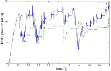
Fig. 15Braking torque waveform
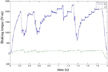
Fig. 16FR speed sine wave and Wigner Ville distribution
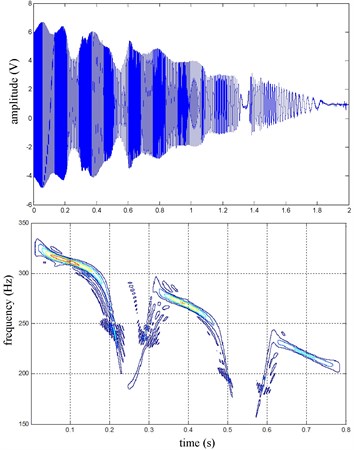
Fig. 17RR speed sine wave and Wigner Ville distribution
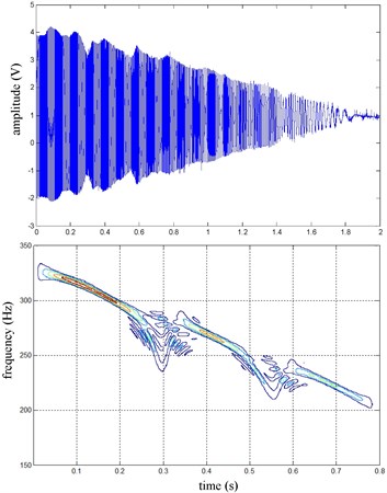
Fig. 18the vehicle velocity and wheel speed
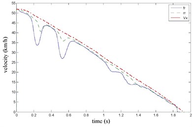
Fig. 19Road friction coefficient identification
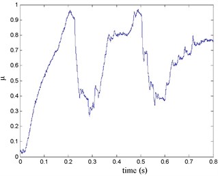
Fig. 20the brake pressure waveform
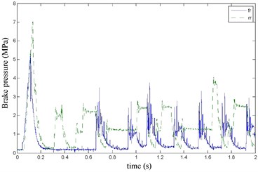
Fig. 21Braking torque waveform
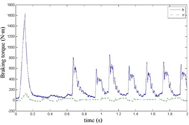
Fig. 22FR speed sine wave and Wigner Ville distribution
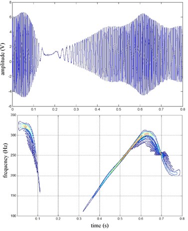
Fig. 23RR speed sine wave and Wigner Ville distribution
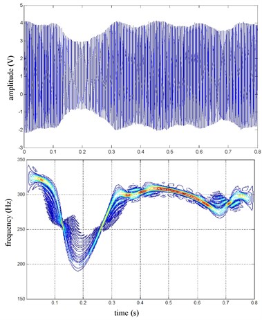
Fig. 24The vehicle velocity and wheel speed
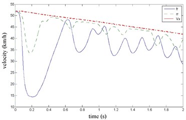
Fig. 25Road friction coefficient identification
3.3.2. Ice road experiment results
The FR and RR wheel brake pressure are shown in Fig. 20 during emergency braking on the ice pavement, and their brake torque are shown in Fig. 21. FR wheel sine waveform and its Wigner Ville distribution are shown in Fig. 22. RR wheel sine waveform and its Wigner Ville distribution are shown in Fig. 23. the vehicle velocity and wheel speed experimental results are shown in Fig. 24, road friction coefficient estimation result by FR wheel signal is shown in Fig. 25. It can be seen the wheel speed control effect is general under high speed on ice road. Wigner Ville distribution is better reflecting the change of the wheel speed (namely its change trend is slower compared with the concrete road as Fig. 17 shown), tire-road friction coefficient estimation precision is good under wheel larger slip rate.
3.3.3. Concrete road→ice road→concrete road experiment results
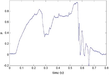
The FR and RR brake pressure are shown in Fig. 26 during emergency braking on the joint road (concrete road→ice road→concrete road), and their brake torque are shown in Fig. 27. FR wheel-speed sine and its Wigner Ville distribution are shown in Fig. 28. RR wheel sine waveform and its Wigner Ville distribution are shown in Fig. 29. The vehicle velocity and wheel speed experimental results are shown in Fig. 30, road friction coefficient estimation result by FR wheel signal is shown in Fig. 31. It can be seen the wheel speed control effect is not satisfactory on joint road, and right front wheel locked at near 0.6 s. the friction coefficient estimation precision is not good on middle low friction road surface and under wheel lock period, but well identified the pavement mutations at near 0.25 s and 0.55 s, that is to say, this method can be used for real-time identification of road mutations.
Fig. 26the brake pressure waveform
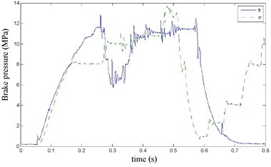
Fig. 27Braking torque waveform
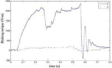
Fig. 28FR speed sine wave and Wigner Ville distribution
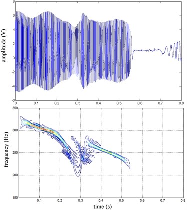
Fig. 29RR speed sine wave and Wigner Ville distribution
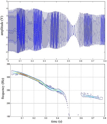
Fig. 30the vehicle velocity and wheel speed
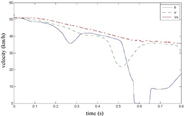
Fig. 31Road friction coefficient identification
4. Conclusions
Due to the interaction mechanism between tire and road is very complex, the multi-freedom rim-beam dynamic model with tire dynamic friction model is set up in this paper. the simulation result shows that the model can well reflect the tire dynamic friction characteristics. the simulation analysis of the key parameters influence characteristics were carried out and the value of each parameter is determined. Then the brake model was established and the calibration experiment of the relationship among the brake pressure, brake torque and braking arm strain voltage signal was carried out. the road friction coefficient estimation model was established, the wheel speed signal conditioning circuit was designed and the measured signal was denoised by the given soft threshold wavelet method. Finally, the vehicle field test was carried out on high friction, low friction and joint road respectively, and the brake pressure, braking torque, vehicle velocity (wheel speed), slip ratio and wheel speed sensor sine wave and its Wigner Ville distribution were collected and analyzed. Tire-road friction coefficient was estimated. the results show that the wheel speed control effect is good on high and low friction road. Wigner Ville distribution well reflected the wheel speed change. the tire-road friction coefficient estimation precision is better when slip ratio is larger. However, wheel speed control effect was not very satisfied on joint road and right front wheel locked occasionally. the tire-road friction coefficient estimation precision was not very satisfied on low friction road surface or during the wheel lock occasionally.
References
-
Erdogan Gurkan, Alexander Lee, Rajamani Rajesh Estimation of tire-road friction coefficient using a novel wireless piezoelectric tire sensor. IEEE Sensors Journal, Vol. 11, Issue 2, 2011, p. 267-279.
-
Shim Taehyun, Margolis Donald Model-based road friction estimation. Vehicle System Dynamics, Vol. 41, Issue 4, 2004, p. 249-276.
-
Ahn Changsun, Peng Huei, TsengH. Eric Robust estimation of road friction coefficient using lateral and longitudinal vehicle dynamics. Vehicle System Dynamics, Vol. 50, Issue 6, 2012, p. 961-985.
-
Lee D. J., Park Y. S. Sliding-mode-based parameter identification with application to tire pressure and tire–road friction. International Journal of Automotive Technology, Vol. 12, Issue 4, 2011, p. 571-577.
-
Erdogan Gurkan, Alexander Lee, Rajamani Rajesh Adaptive vibration cancellation for tire-road friction coefficient estimation on winter maintenance vehicles. IEEE Transactions on Control Systems Technology, Vol. 18, Issue 5, 2010, p. 1023-1032.
-
Rajamani Rajesh, Phanomchoeng Gridsada, Piyabongkarn Damrongrit, Lew Jae Y. Algorithms for real-time estimation of individual wheel tire-road friction coefficients. IEEE/ASME Transactions on Mechatronics, Vol. 17, Issue 6, 2012, p. 1183-1195.
-
Wang Rongrong, Wang Junmin Tire-road friction coefficient and tire cornering stiffness estimation based on longitudinal tire force difference generation. Control Engineering Practice. Vol. 21, Issue 1, 2013, p. 65-75.
-
Alvarez Luis, Yi Jingang, Horowitz Roberto, Olmos Luis Dynamic friction model-based tire-road friction estimation and emergency braking control. Transactions of the ASME. Vol. 127, Issue 1, 2005, p. 22-32.
Cited by
About this article

This research was supported by the Key Programs for Science and Technology Development of Henan Province (No. 122102210045), the National Undergraduate Training Programs for Innovation and Entrepreneurship (No. 201510460001) and Henan Polytechnic University Education Teaching Reform Research Projects (No. 2015JG034).
Xiao-bin Fan: overall design and thesis writing. Bing-xu Fan: tire dynamic characteristics research and modeling. Feng Wang: measurement and control circuit design and system development. Qun-sheng Xia: planning experiment scheme and implementation. Ping-an Wang: the experimental operation and data processing.
