Abstract
The tuned mass damper parameters designing for structural systems based on combining linear matrix inequality with genetic algorithm is of concern in this paper. Firstly, based on matrix transform, the novel model description with a singular style for structural systems is obtained, in which the possible coupling of those uncertainties is avoided. Secondly, an approach, which combines linear matrix inequality with genetic algorithm, is taken in this work to solving the optimization problems, and the optimized tuned mass damper parameters can be obtained by solving the optimization problems such that the tuned-mass-damper-controlled systems have a prescribed level of vibration attenuation performance. Furthermore, the obtained results are also extended to the uncertain cases. Finally, the effectiveness of the obtained theorems is demonstrated by numerical simulation results.
1. Introduction
Since the concept of structural control was proposed by Yao et al. in 1972 [1], the research on structural control has been conducted by many scholars, and great strides have been made in advancing the theory and practice in this area. Generally speaking, the existing results can be classified into three types: passive control (without external energy input), semi-active or active control (need energy input) and intelligent-algorithm-based intelligent control [2, 3]. Active control can achieves a satisfying control result [4, 5], however, it needs continuous external energy supply which results in its low reliability. On the contrary, passive control needs no external energy input, thus, it can reach a much higher reliability. Tuned Mass Damper (TMD), as one kind of passive control device, has received considerable attention for its virtues, such as no energy consumption, low cost, easy installation, etc., and many results about TMD control have been achieved during the last decades, for example, the Trans-Tokyo Bay Highway Crossing, completed in1997, is 11 km in total length, and the vibration was significantly reduced by TMDs inside the box girder [6]. In order to diminish the vibrations in the structure during earthquakes and typhoons, the main tower of the Akashi-Kaikyo suspension bridge also contains TMDs [7]. There were two buildings in U.S. equipped with TMD, one is Citicorp Center, New York and the other is John Hancock Tower, Boston [8]. Moreover, 18 vertical and 18 lateral TMDs were installed in Dubai Meydan Racecourse Stadium to control the vibration induced by wind load in the two directions, and the results demonstrated a substantial reduction of the vertical and lateral wind vibration [9]. Some more achievements about TMD control can be found in [10-17] and those references therein. The TMD system is a well-accepted device for controlling flexible structures, particularly, tall buildings [10-12]. However, to the best of the authors’ knowledge, most of the TMD applications have been made towards mitigation of wind-induced motion, and seismic effectiveness of TMDs still has not been fully investigated. A typical kind of TMD consists of a mass block, a viscous damper and a spring connected to the main structure. The natural frequency of the TMD is tuned to the resonant frequency of the main structure, so, a large amount of entrance energy is transferred to the TMD [18]. Obviously, the performance of the TMD is based on the design of its parameters: mass, stiffness, and damping ratio.
The most common TMD designing methods are LQR, LQG, sliding mode control, pole assignment, control, energy-to-peak control, fuzzy control, and so on [19-23]. Moreover, in order to achieve a better control performance, some optimization techniques are often used in optimizing those TMD parameters [4, 10, 24-26]. Such as, in [10], the parameters of the TMD were optimally designed using multi-objective genetic algorithms for a 12-story realistic building through both deterministic and robust design procedures. Yang et al. proposed an innovative practical approach to optimally design the TMD system in [26], and the effectiveness was illustrated by examples. It is worth pointing out that genetic algorithm has some virtues, such as global genetic optimization etc., and has been widely used for the parameter optimization in control systems. On the other hand, in recent years, LMI technique is widely researched and used in the system stability analysis and controller design. For example, based on LMI, references [27, 28] concerned the vibration-attenuation controller design for linear structure systems. In terms of LMI, Wu et al. [29] discussed the admissibility and dissipativity of singular systems, and some improved results were obtained. Some more results about LMI can be found in [30-32] and those references therein. Although the LMI technique has been widely used in the system stability analysis and controller design, LMI-based TMD parameters design also has not been fully investigated. Thus, there is still much room for improvement in this important issue.
In this paper, the parameters of the TMD will be optimized by combining LMI technique with genetic algorithm. First, the novel model description for uncertain structural systems is obtained by introducing the singular system description, in which the coupling of uncertainties is avioded when the mass, damping and stiffness are subjected to possible perturbations. Then, in terms of combining LMI technique with genetic algorithm to solve the optimization problem, the optimized TMD parameters can be easily achieved such that the TMD-controlled system has a prescribed level of vibration attenuation performance, and the obtained results are also extended to the uncertain cases. In the end, the effectiveness of the obtained theorems is illuminated by numerical examples.
Notation: Throughout this paper, for real matrices and , the notation (respectively, ) means that the matrix is semi-positive definite (respectively, positive definite). is the identity matrix with appropriate dimension, and is the identity matrix. and represent the zero matrix and the -dimensional zero vector, respectively. The superscript “” represents transpose. expresses the 2-norm of . We define . For a symmetric matrix, denotes the symmetric terms. The symbol stands for the-dimensional Euclidean space, and is the set of real matrices.
2. Problem formulation and dynamic models
Consider andegree-of-freedom structural system with TMDs installed on storeys respectively, which are shown in Fig. 1, where , and are the mass, damping and stiffness of storey, respectively; , and are the mass, damping and stiffness of TMD, respectively. The structural system subjected to horizontal earthquake excitation can be expressed in the following model equations:
where:
Fig. 1n degree-of-freedom structural system controlled by TMDs
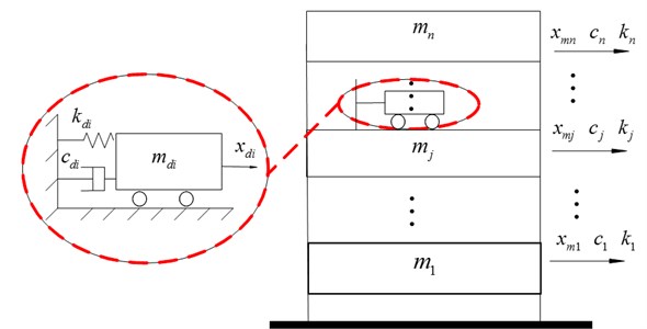
, , , are the mass, damping and stiffness matrices of the structure, respectively. is the external excitation vector. , is the relative displacement of storey to the ground, donates the relative displacement of the TMD to the storey , on which the TMD is installed. is a vector with the th item to be 1 and others to be 0, which means TMD is installed on storey . Based on Eqs. (1)-(2), the following system equation is obtained:
where denote the relative displacement of the th TMD to the ground. Obviously , and:
In terms of Eq. (3), it is easy to obtain the following singular description of the system model:
where , is a problem based matrix with suitable dimension, and:
Consider the uncertainties existing in the mass, damping and stiffness matrices of the structural systems, and the uncertainties satisfy , , , , , , where 1, 2,…, , 1, 2,…, , and . 1, 2,…, , while 1, 2, 3, and 1, 2,…, , while 4, 5, 6. Then, the uncertain structural systems can be expressed in the following form:
where:
Remark 1: It has been shown in the references [13, 33] that the linear structural system Eq. (3) can be described in the following state equation:
where:
It is obvious that there exists a coupling of the uncertainties when the mass, damping and stiffness are subjected to possible perturbations, for example, while uncertainties exist in the matrices and , the uncertain description of the matrix block can be expressed as , which results in a serious conservatism in the system analysis and synthesis obviously, however this is not existing in the state Eq. (5). That is to say, Eq. (5) has less conservatism than Eq. (6).
Lemma 1 [34]: given matrices , and with appropriate dimensions and with symmetrical, then holds for any satisfying , if and only if there exists a scalar such that .
In the following content, we consider how to obtain the suitable TMD parameters such that the system with the designed TMDs has a satisfying disturbance attenuation performance. Then, the robustness of the TMD control system will be considered.
3. TMD parameters design for structural systems
Theorem 1: The system Eq. (4) is admissible with performance for all non-zero , and constant , if there exist a positive definite symmetric matrix and matrix satisfying the following matrix inequality:
where is any full-column rank matrix satisfying .
Proof:First, system Eq. (4) is regular and impulse free under the condition of Theorem 1 is proved. Form Eq. (7), we have:
According to [35], it can be obtained that the system (4) is regular and impulse free. Then, system Eq. (4) is stable under the condition of Theorem 1 will be shown. Choose a Lyapunov functional candidate as:
The derivative of along the trajectories of Eq. (4) satisfies:
Noting , we obtain:
Next, the performance of the system under zero initial condition (, and ) will be established. Consider the following index:
Then, for any non-zero , there holds:
Noting Eqs. (10)-(13), after some algebraic manipulations, the following results can be obtained:
Then, is obtained from Eq. (7). Thus , and is satisfied for any non-zero . Assume the zero disturbance input, i.e. . If , it is easy to obtain , and the asymptotic stability of system Eq. (4) is established. This completes the proof.
Remark 2: The optimal TMD parameters can be obtained by solving the following optimization problems, such as, according to solving the optimization 1, the TMD parameters, which guarantee the minimum , can be obtained. For a given ( is a constant), a set of TMD parameters, which has the minimum TMD masses, is obtained by solving the optimization 2.
Optimization 1:
Optimization 2:
Theorem 2: The system Eq. (5) is robustly admissible with performance for all non-zero , and constant , if there exist positive definite symmetric matrix , matrix and positive scalars , satisfying the following LMI:
where is any full-column rank matrix satisfying , and:
Proof: Replacing and with and , Eq. (7) can be expressed as:
By Lemma 1, Eq. (18) holds if and only if there exist positive scalars (1, 2, 3), , such that:
Applying the Schur complement, equation (17) is equivalent to equation (19). This completes the proof.
Obviously, the optimal TMD parameters for the uncertain systems can be obtained by solving the following optimization problems.
Optimization 3:
Optimization 4:
Remark 3: It is worthy to point out that there exist nonlinear properties in Eq. (7) and (17) for the coupling of the parameters , , (1, 2,…, ) with the matrices and . Thus, the traditional LMI solving methods is useless to solve Eq. (7) and (17). Fortunately, there are lots of intelligent algorithms (such as, genetic algorithm, neural network, particle swarm optimization and ant colony algorithm, etc.), which have been certified to be effective for treating the nonlinear properties of all kinds of equations. In this paper, a method of combining genetic algorithm with LMI toolbox is introduced to solve the optimizations 1 to 4, and the algorithm is shown as following:
Algorithm.
Step 0 (initialization): Set the maximum iteration step , population size , crossover rate , mutation rate , and the steps counter . Then, the individual solutions are randomly generated to form an initial population, for example, in optimization 1, the population size is , that is, the initial population are , , , 1, 2,…,, 1, 2,…,.
Step 1 (fitness of the individual solutions): The fitness is the value of the objective function in the optimization problem being solved. Based on solving of the optimization 1, 2, 3 or 4, the fitness of the individual solutions can be obtained.
Step 2 (selection, reproduction and mutation): The more fit individuals are stochastically selected from the current population, and each individual’s genome is modified (recombined and possibly randomly mutated) to form a new generation. The new generation of candidate solutions is then used in the next iteration of the algorithm.
Step 3 (production of the new generation): Based on solving of the optimization 1, 2, 3 or 4, the fitness of the individuals in the new generation can be obtained, and according to fitness of the individuals in the new generation, the candidate individual solutions can be obtained and then used in the next iteration of the algorithm.
Step 4 (Termination): The algorithm terminates when , or a maximum number of generations has been produced, or a satisfactory fitness level has been reached for the population, and the individual solution with the maximum fitness is chosen as the optimal solution. Otherwise, set , and go back to step 2.
4. Illustrative example
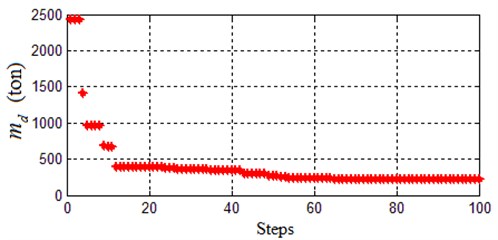
Consider a 3 degree-of-freedom structural system, which has a TMD installed on the third storey. The structural parameters are as following: 345.6 ton, 2973 kNs/m-1, 3.404×10⁵ kN/m, 1, 2, 3, are the mass, damping and stiffness of each storey respectively [19]. , and , which are the parameters of the TMD, need to be designed. Choose as the controlled output, that is, . Firstly, the system without uncertainties is considered. Set 0.5, and choose the minimum as the optimization objective. Then, by setting the maximum iteration step 100, we use the Matlab GAOPT Toolbox to solve the Algorithm mentioned above (the values of obtained in the iteration are shown in Fig. 2), and obtain the optimal TMD parameters, which are shown in Table 1. For description in brevity, this TMD is denoted as TMD1 thereafter.
Table 1The final results after 100 steps
21244.88 | 2632.25 | 218.28 | 0.5 |
Fig. 2The md obtained in the iteration
In order to verify the dynamics of the TMD-controlled system, a time history of acceleration from North Korea seismic excitation is applied to this system (see Fig. 3, http://www. vibrationdata.com/newsletters.html), and the storey 3’ displacements of the system with and without TMD1 are shown in Fig. 4. The displacements of the other two storeys and the velocities of three storeys have a similar varying trend, which is omitted here for brevity. It is shown from Fig. 4 that TMD 1 is effective in attenuating the vibration of the structural systems. The maximum displacements and velocities of the three storeys are shown in Table 2. The Percentage of the Maximum-displacement-reduced Value (PMV) of the system with TMD1 is ((0.0599-0.0185))/0.0599 ≈ 33.06 % in storey 1, and the other PMVs are shown in Table 2. That is, the maximum displacements and velocities are all attenuated when the system is controlled by TMD1. Thus, the effectiveness of TMD1 is obvious.
Fig. 3North Korea seismic excitation
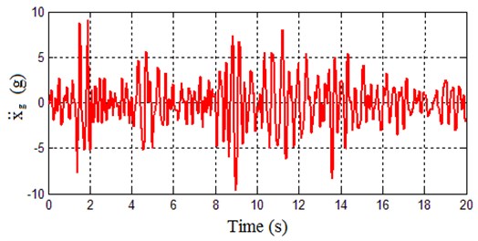
Fig. 4The storey 3’ displacements of the structural system
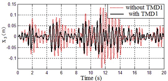
Table 2the maximum displacements and accelerations of the structural system
Displacements (m) | Velocities (m/s) | |||||
Floor 1 | Floor 2 | Floor 3 | Floor 1 | Floor 2 | Floor 3 | |
Without TMD1 | 0.0599 | 0.1078 | 0.1348 | 0.9108 | 1.6771 | 2.1212 |
with TMD1 | 0.0401 | 0.0775 | 0.1019 | 0.5594 | 1.0249 | 1.3168 |
PMV | 33.06 % | 28.11 % | 24.41 % | 38.58 % | 38.89 % | 37.92 % |
Then, the uncertain case is considered. Consider the uncertainties as applied to the mass, stiffness and damping coefficients of the first storey, and assume the parameter uncertainties satisfying , , , , , . Choose the minimum as the optimization objective. By setting the maximum iteration step 50, we use the Matlab GAOPT Toolbox to solve the Algorithm mentioned above (the values of obtained in the iteration are shown in Fig. 5), and obtain the TMD parameters which are shown in Table 3. For description in brevity, this TMD is denoted as TMD2 thereafter.
Table 3The final result after 50 steps in the uncertain case
7135.642 | 7797.655 | 1620.312 | 0.302577 |
Under the excitation mentioned above, the displacements of storey 3 for the system with TMD2 are shown in Fig. 6. The displacements of the other two storeys and the velocities of the three storeys have a similar varying trend, which is omitted here for brevity. It is shown from Fig. 6 that TMD 2 is effective in attenuating the vibration of the uncertain structural systems obviously. The maximum displacements and velocities of the three storeys are shown in Table 4. From Table 4, it is easy to get that the maximum displacements and velocities are all attenuated when the system is controlled by TMD2. Thus, it is validated that TMD2 is robust to parameter uncertainties.
Table 4The maximum displacements and accelerations of the uncertain structural system
Displacements (m) | Velocities (m/s) | |||||
Floor 1 | Floor 2 | Floor 3 | Floor 1 | Floor 2 | Floor 3 | |
Without TMD2 | 0.0643 | 0.1061 | 0.1290 | 1.0542 | 1.5584 | 1.8664 |
With TMD2 | 0.0226 | 0.0413 | 0.0570 | 0.3583 | 0.6283 | 0.8277 |
PMV | 64.85 % | 61.07 % | 55.81 % | 66.01 % | 59.68 % | 55.65 % |
Fig. 5The γ obtained in the iteration for the uncertain case
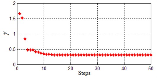
Fig. 6The storey 3’ displacements of the uncertain structural system
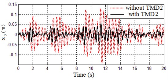
Table 5The maximum displacements and accelerations of the uncertain structural system
Displacements (m) | Velocities (m/s) | |||||
Floor 1 | Floor 2 | Floor 3 | Floor 1 | Floor 2 | Floor 3 | |
Without TMD2 | 0.0098 | 0.0189 | 0.0240 | 0.1488 | 0.2748 | 0.3579 |
With TMD2 | 0.0084 | 0.0138 | 0.0195 | 0.0713 | 0.1321 | 0.1786 |
PMV | 14.29 % | 26.98 % | 18.75 % | 52.08 % | 51.93 % | 50.10 % |
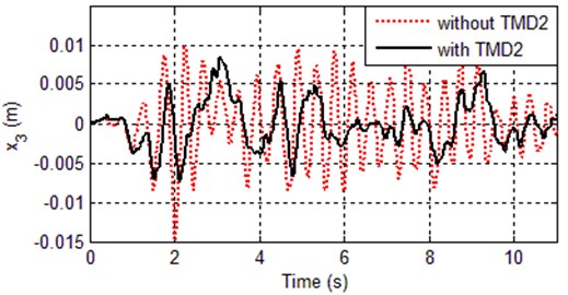
In order to further verify the effctiveness of the obtained TMD controller, another seismic excitation (see Fig. 7), which was adopted as an excitation in [2, 19-21], is applied to this system. The storey 3’ displacements of the system with and without TMD2 are shown in Fig. 8. The displacements of the other two storeys and the velocities of three storeys have a similar varying trend, which is omitted here for brevity. It is shown from Fig. 8 that TMD 2 is still effective in attenuating the vibration of the uncertain structural systems which is excited by the seismic excitation shown in Fig. 7. The maximum displacements, velocities and PMVs of the three storeys are shown in Table 5. From Table 5, it is easy to get that the maximum displacements and velocities are all attenuated when the system is controlled by TMD2. Thus, the effectiveness of TMD2 is validated again.
Fig. 7EI Centro 1940 earthquake excitation
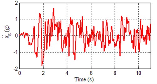
Fig. 8The storey 3’ displacements of the uncertain structural system
5. Conclusions
The TMD parameters designing for structural systems based on combining LMI technique with genetic algorithm is of concern in this paper. Firstly, based on matrix transform, the singular description of the structural systems controlled by TMDs is obtained. Secondly, in terms of combining LMI toolbox with genetic algorithm to solving the optimization problem, the optimized TMD parameters are obtained such that the TMD-controlled system has a prescribed level of vibration attenuation performance. Thirdly, the obtained results are also extended to the uncertain cases. Finally, examples are given to show the effectiveness of the obtained theorems.
References
-
Yao J. Concept of structural control. Journal of Structural Division, Vol. 98, Issue 7, 1972, p. 1567-1574.
-
Weng F., Ding Y., Liang L., Yang G., Ge J. Finite-time vibration-attenuation controller design for structural systems with actuator faults and parameter uncertainties. Journal of Vibration Engineering and Technologies, Vol. 4, Issue 2, 2016, p. 117-129.
-
Soong T., Cimellaro G. Future directions in structural control. Structural Control and Health Monitoring, Vol. 16, Issue 1, 2009, p. 7-16.
-
Du H., Zhang N., Samali B., Naghdy F. Robust sampled-data control of structures subject to parameter uncertainties and actuator saturation. Engineering Structures, Vol. 36, 2012, p. 39-48.
-
Ding Y., Weng F., Tang M., Ge J. Active vibration-attenuation controller design for uncertain structural systems with input time-delay. Earthquake Engineering and Engineering Vibration, Vol. 14, Issue 3, 2015, p. 477-486.
-
Fujino Y. Vibration, control and monitoring of long-span bridges-recent research, developments and practice in Japan. Journal of Constructional Steel Research, Vol. 58, Issue 1, 2002, p. 71-97.
-
Koshimura K., Tatsumi M., Hata K. Vibration control of the main towers of the Akasi Kaikyo Bridge. Proceedings of the First World Conference on Structural Control, Los Angels, California, Vol. 2, 1994, p. 98-106.
-
Ou J., Wu B. Recent advances in research on and applications of passive energy dissipation Systems. Earthquake Engineering and Engineering Vibration, Vol. 16, Issue 3, 1996, p. 72-96.
-
Chen Y., Cao T. Tune mass damper system for roof wind control of Meydan Racecourse Stadium in Dubai. Building Structure, Vol. 42, Issue 3, 2012, p. 49-53.
-
Pourzeynali S., Salimi S., Kalesar H. Robust multi-objective optimization design of TMD control device to reduce tall building responses against earthquake excitations using genetic algorithms. Scientia Iranica, Vol. 20, Issue 2, 2013, p. 207-221.
-
Morga M., Marano G. Optimization criteria of TMD to reduce vibrations generated by the wind in a slender structure. Journal of Vibration and Control, Vol. 20, Issue 16, 2014, p. 2404-2416.
-
Yang Y., Dai W., Liu Q. Design and implementation of two-degree-of-freedom tuned mass damper in milling vibration mitigation. Journal of Sound and Vibration, Vol. 335, Issue 20, 2015, p. 78-88.
-
Debnath N., Deb S., Dutta A. Multi-modal vibration control of truss bridges with tuned mass dampers under general loading. Journal of Vibration and Control, 2015, p. 1-20.
-
Xiang P., Nishitani A. Seismic vibration control of building structures with multiple tuned mass damper floors integrated. Earthquake Engineering and Structural Dynamics, Vol. 43, 2014, p. 909-925.
-
Soto M., Adeli H. Optimum tuning parameters of tuned mass dampers for vibration control of irregular highrise building structures. Journal of Civil Engineering and Management, Vol. 20, Issue 5, 2014, p. 609-620.
-
Zhou D., Li J., Hansen C. Suppression of the stationary maglev vehicle-bridge coupled resonance using a tuned mass damper. Journal of Vibration and Control, Vol. 19, Issue 2, 2013, p. 191-203.
-
Lin G., Lin C., Chen B., Soong T. Vibration control performance of tuned mass dampers with resettable variable stiffness. Engineering Structures, Vol. 83, 2015, p. 187-197.
-
Wang A., Lin Y. Vibration control of a tall building subjected to earthquake excitation. Journal of Sound and Vibration, Vol. 299, 2007, p. 757-773.
-
Du H., Zhang N. H∞ control for buildings with time delay in control via linear matrix inequalities and genetic algorithms. Engineering Structures, Vol. 30, Issue 1, 2008, p. 81-92.
-
Zhang W., Chen Y., Gao H. Energy-to-peak control for seismic-excited buildings with actuator faults and parameter uncertainties. Journal of Sound and Vibration, Vol. 330, Issue 4, 2011, p. 581-602.
-
Samali B., Al-Dawod M. Performance of a five-story benchmark model using an active tuned mass damper and a fuzzy controller. Engineering Structures, Vol. 25, 2003, p. 1597-1610.
-
Li L., Song G., Ou J. Nonlinear structural vibration suppression using dynamic neural network observer and adaptive fuzzy sliding mode control. Journal of Vibration and Control, Vol. 16, Issue 10, 2010, p. 1503-1526.
-
Rathi A., Chakraborty A. Robust design of TMD for vibration control of uncertain systems using adaptive response surface method. Advances in Structural Engineering, 2015, p. 1505-1517.
-
Aldermir U. Optimal control of structures with semiactive tuned mass dampers. Journal of Sound and Vibration, Vol. 266, Issue 4, 2003, p. 847-874.
-
Alexandros A. Optimal probabilistic design of seismic dampers for the protection of isolated bridges against near-fault seismic excitations. Engineering Structures, Vol. 33, Issue 12, 2011, p. 3496-3508.
-
Yang F., Sedaghati R., Esmailzadeh E. Optimal design of distributed tuned mass dampers for passive vibration control of structures. Structural Control and Health Monitoring, Vol. 22, Issue 2, 2015, p. 221-236.
-
Ding Y., Weng F., Ge J., Nguyen J. Displacement-constrained vibration-attenuation controller design for linear structure systems with parameter uncertainties. International Journal of Computer Applications in Technology, Vol. 53, Issue 1, 2016, p. 82-90.
-
Ding Y., Weng F., Jiang X., Tang M. Vibration-attenuation controller design for uncertain mechanical systems with input time delay. Shock and Vibration, 2016, p. 9686358.
-
Wu Z., Park J., Su H., Chu J. Admissibility and dissipativity analysis for discrete-time singular systems with mixed time-varying delays. Applied Mathematics and Computation, Vol. 218, Issue 13, 2012, p. 7128-7138.
-
Ahmadi A., Aldeen M. An LMI approach to the design of robust delay-dependent overlapping load frequency control of uncertain power systems. International Journal of Electrical Power and Energy Systems, Vol. 81, 2016, p. 48-63.
-
Long S., Zhong S. H∞ control for a class of discrete-time singular systems via dynamic feedback controller. Applied Mathematics Letters, Vol. 58, 2016, p. 110-118.
-
Wu Z., Shi P., Su H., Lu R. Dissipativity-based sampled-data fuzzy control design and its application to truck-trailer system. IEEE Transactions on Fuzzy Systems, Vol. 23, Issue 5, 2015, p. 1669-1679.
-
Karimi H., Zapateiro M., Luo N. An LMI approach to vibration control of base-isolated building structures with delayed measurements. International Journal of Systems Science, Vol. 41, Issue 12, 2010, p. 1511-1523.
-
Weng F., Ding Y., Liang L. Acceleration-based vibration control for structural systems with actuator faults and finite-time state constraint. Noise and Vibration Worldwide, Vol. 46, Issue 4, 2015, p. 10-21.
-
Dai L. Singular control systems. Lecture Notes in Control and Information Sciences, Springer-Verlag, New York, 1989.
Cited by
About this article

This research has been supported by the National Natural Science Foundation (No. 61463018), Jiangxi Provincial Natural Science Foundation (No. 20151BAB207046) and the Natural Science Foundation of Jiangxi University of Science and Technology (No. NSFJ2014-K16) of China.
