Abstract
Based on the heat-to-sound and virtual-source principles developed in previous works, this paper designs a thermoacoustic traducer for measurement of fast-time heatflux from/to heating/cooling sources. The inverse thermoacoustic algorithm in this instrumentation is fulfilled by a PID-adaptive Luenberger observer, which is newly developed here. It is able to real-time measure the heatflux with oscillating frequency larger than 10 Hz, beyond the capability of thermoelectric sensors. Such an elegant performance is then utilized to clarify the following two doubts: one is about the ad hoc energy-transfer process in self-excited thermoacoustics, and the other is for the existence of thermal-inductance materials in nature
1. Introduction
The heat-to-sound principle explains how a heatflux into an air tube can drive acoustic waves [1, 2]. That is, on the interface of heating source and the air tube, the heatflux gives rise to entropy-rate that changes the fluid density-rate there, which initiates acoustic velocity due to mass continuity. With such an acoustic source on the boundary, acoustic-pressure is then developed inside the whole tube. Therein the boundary inhomogeneity specified by the heatflux can be virtually realized as a delta source of heat generation on the interface. A detailed exploration on this realization can refer to [1]. With this realization, the dynamics from the heatflux to the acoustic pressure can be modelled as an input-output relationship. This input-output model can easily be identified in the Laplace domain, based on which an input-state observer can be designed to real-time measure the heatflux with an acoustic-pressure sensor. This input-state observer can be programmed into a dsPIC controller with Euler discretization [3], and then works as an inverse thermoacoustic algorithm to online deduce the heatflux. Besides the air tube and a circuit board that implements the inverse thermoacoustic algorithm, the thermoacoustic transducer comprises a porous media with ultra-low thermal-resistance to allow for measurement of the heatflux into a cooling source.
It is popular in industry and academy to measure heatflux through thermoelectric traducers, such as thin-film sensors, Gardon sensors, and coaxial thermocouples. They measure temperature gradients from electric-resistance variations. To measure powerful heatflux, Gardon heatflux sensor usually includes a costly water-cooling heat-sink. For faster measurement, the coaxial thermocouple was developed as a new material to replace thin films. For real-time measurements, these sensors are embedded with the inverse heat-transfer programs that calculate the heatflux source out of temperature signals [4-6]. Even so, it was found that thermoelectric transducers show incapability of measuring high-frequency (say 10 Hz) or impulsive fluctuations of heatflux, since temperature-to-electric materials are ultra-low-pass filters in nature. For modern practices of thermo science and engineering, reliable measurements of fast-time heatflux are needed, for example, the access to the transient behavior of thermally inductive materials that store entropy-flow inside [7, 8]. Therefore, in this paper is the thermoacoustic transducer developed to solve the situation upon fast-time measurement of heatflux.
Of the thermoacoustic transducer, the inverse thermoacoustic algorithm (ITAA) is analogous to the inverse heat-conduction problems (IHCP) of thermoelectric transducers. There are three types of IHCP methodologies in this decade: inverse filter solutions in Laplace domain [9-13], Luenberger input-state observers based on state-space models [14], and neural networks back-propagated trained to do the inverse [15]. Among these, the neural networks are intelligent but with the trade-off of reliability. The inverse filters are sensitive, but suffer noises and uncertainties from improper transfer-functions and initial conditions, respectively. Luenberger observers, such as Kalman filters, become rather conservative for nonlinear dynamics, although they are excellent in rejection of noises and uncertainties. Since the thermoacoustic dynamics can be considered as a linear process, Luenberger state-input observer is chosen here as the methodology for the ITAA design as to accommodate reliability, sensitivity, and rejection of noises and uncertainties.
Luenberger observer is originally developed to estimate the state as the input can be online measured and sent into the observer [16]. To extend the Luenberger observer to estimate unknown inputs, the state equation can be expanded to contain the dynamics of the to-be-estimated input [17]. For the reduction of steady-state error of state estimation, the observer gain can be extended to be a proportion-integral (PI) type from the proportional (P) type [18]. To shorten the transience in the input estimation, the dynamics of to-be-estimated input can be replaced by adaptive approaches such as the gradient rule [19]. Therefore, for simultaneous reduction of steady-state error and transient time of state estimation, unknown input PI observers combined with the adaptive approaches were developed in, say, [20]. In fact, the gradient rule can be extended to be a proportion-integral (PI) type from the proportional (P) type, to further suppress the steady-state error of input estimation. In this work, the inverse thermoacoustic algorithm is virtually a Luenberger state-input observer combined with proportion-integral-derivative (PID) gradient rule that further improves both of the steady-state and transient performance of input estimation. It is found from the experiments that such a PID-adaptive Luenberger works well for ITAA.
Including this section, this paper is organized into five sections. In Section 2 is the design of thermoacoustic transducer, based on the heat-to-sound and virtual-source principles. Section 3 synthesizes the inverse thermoacoustic algorithm structured as a PID-adaptive Luenberger observer. Section 4 applies the inverse thermoacoustic algorithm to measure the heatflux oscillations in a self-excited thermoacoustic engine, and to verify the existence of thermal inductance.
2. Thermoacoustic transducers
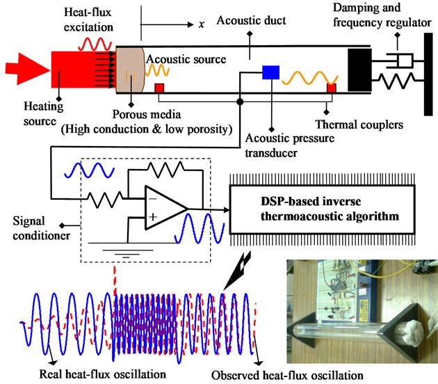
The thermoacoustic transducer designed for measuring fast-time heatflux is plotted in Fig. 1. It is assembled by a porous media, an air tube, an acoustic damper, an acoustic-pressure sensor, two thermocouples, and a circuit board for signal processing.
In the interface between the air tube and the porous media, , the to-be-measured heatflux flows into the air tube. Based on energy conservation, the heatflux on the boundary can be realized into a delta heat-generation in conjunction with a Robin homogeneous boundary, which keeps the acoustic dynamics inside the tube almost the same. Based furthermore on the heat-to-sound principle in [1], on the boundary this virtual heat-generation gives rise to entropy-rate that changes density-rate thereon, which initiates acoustic velocity at . Due to the inertia and stiffness of fluid fluctuation, traveling wave or standing wave of acoustic pressure is developed inside the air tube. That is, in the virtual-source realization, the heatflux becomes an input rather than a part of boundary condition. Let the acoustic-pressure at some location is online measured, and denoted by . The dynamics from the input to the output will be identified in Laplace domain. This input-output model serves for the synthesis of state-input observer that plays as the inverse thermoacoustic algorithm (ITAA).
The function of porous media is to allow for reverse acoustic-velocity across the boundary, while the heat flows into a cooling source from the air tube. To decrease the difference between the heatflux out of heating source and that into the air-tube, the porous media is of ultra-low thermal-resistance and porosity. The mass-spring-damper attached to the tail of air tube has the purpose of model regulation. The damper is for decreasing the number of dominated acoustic-modes, the mass is for amplifying the frequency responses in low-frequency region, and the spring is to suppress the mean-flow effect. As for the circuit board, it comprises analog circuits for signal conditioning and a Microchip-dsPIC chip that implements the ITAA.
Fig. 1Real time measurement of surface heat-flux oscillations with thermoacoustic transducer embedded with inverse thermoacoustics
As for the identification of the dynamics from the input to the output , it is a routine work in control engineering, referring to [2], which is proceeded as follows:
Step 1: Give an input being able to be measured by a thin-film heatflux sensor, and collect the responses of .
Step 2: Calculate the frequency spectrums of and , denote them by and . The frequency response of the dynamics is .
Step 3: The transfer-function of the dynamics , , can be obtained through curve-fitting of its frequency response ) in the Bode plot.
Step 4: Derive an observable state-space realization of , such as the observability canonical form. Choose a proper sampling-time , and discretize this state-space model to be:
where represents the state vector, the cardinality of which is identical to the order of the identified dynamics .
3. Inverse thermoacoustic algorithm
The next task is to develop the dynamics that is capable of deducing the boundary heatflux from the pointed sensing of acoustic pressure based on the identified dynamics in Eq. (1). These dynamics plays as an online inverse of the forward dynamics , named here by Inverse Thermoacoustic Algorithm (ITAA). As mentioned in the introduction section, several online-inverse processes were ever derived for inverse heat-conduction problems and others, among which many researchers like the method of inverse transfer-function. Here the inverse transfer-function must be improper, i.e. the order of denominator is larger than that of the nominator, so that significant noises will arise from online differentiation. Moreover, the method of inverse transfer-function treats the initial state as modelling uncertainty, which also severely affects measurement accuracy. On the other hand, this work improves the Luenberger state-input observer with PID adaptive to obtain an online-inverse attributed to reliability, sensitivity, and rejection of noises and uncertainties.
In the sequel is the ITAA programmed into a dsPIC-controller. Denote the estimated state and the estimate input by and , respectively, Make a guess of initial state and input, and . At the present time , within a sampling period , two consecutive stages are coded as follows:
Stage 1: Luenberger observer for state estimation:
where the represents the update of estimated state for the next instant. The observer-gain is chosen such that is Hurwitz, i.e. all of its eigenvalues are inside the unit circle in the complex plane. Specially, Kalman-filtering gains are all candidates.
Stage 2: Gradient rule for input estimation:
where the represents the update of estimated input for the next instant . Therein stands for the error away from dynamic equality, for the summation of errors in history, and for the difference of errors at two consecutive instants. The parameters represent the to-be-adjusted PID-gains that are positive definite.
Subtraction Eq. (2) from Eq. (1) yields:
where is Hurwitz. Suppose the estimated input coincides with the real input at some time, then the estimated state will converge to the real state with the transience determined by the eigenvalues of . This explains the rationale of Eq. (2). During the choice of an observer-gain , note that there is always a trade-off between fast convergence and rejection of sensor noises.
The information of the identified plant in Eq. (1) can be utilized again to update the estimated input by adaptive approaches. At every instant the update of the estimated input is to minimize the 2-norms of the error defined in Eq. (3a). That is:
where is known as the dynamic parameter in the gradient rule. Eq. (5) can be rephrased as:
where is the proportional gain of the gradient rule. To improve the transient performance and reduce the steady-state error, we can add a derivative gain and an integral gain , respectively, to the gradient rule, such that:
which is just the Eq. (3d). As for the choice of PID gains in this PID-gradient rule, we can let the P-gain coarsely adjust the response, and then finely tune the I-gain for zero steady-state error and the D-gain to shorten the converging time. This PID-gradient rule is newly developed in this paper, which works especially well for measurement of fast-time heatflux, as shown in the sequel.
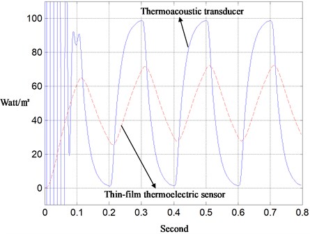
The thermoacoustic transducer depicted in Fig. 1 and the ITAA presented in Eqs. (2) and (3) are then put into a pilot-run. Therein an electrically heating source is on-off switched by a buck chopper to excite heatflux into the air-tube. A purchased thin-film thermoelectric sensor and the self-designed thermoacoustic transducer are taken to real-time measure the heatflux on the boundary. As the switching frequency of the heating source is as low as 1 Hz, the thermoacoustic transducer with the sampling-time 0.001 sec and the PID-gains of gradient rule (8000, 0.3, 8000) performs almost as well as the thin-film heatflux sensor, as shown in Fig. 2. However, as the switching frequency is increased to 5 Hz, it becomes obvious that the thermoelectric sensor is unable to catch such a fast-time heatflux. This fact is shown in Fig. 3, which verifies the value of this new sensor applied to modern thermo-industry.
Fig. 2Measurement of slow-time heat-flux with thermoelectric transducer for system identification and for verification of inverse thermoacoustic algorithm
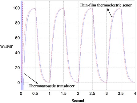
Fig. 3Measurement of fast-time heat-flux with thermoacoustic and thermoelectric transducers
Besides the Luenberger observer teamed with the PID-gradient rule, a white-noise filter is always programmed into the embedded controller. Therein, the acoustic-pressure signal sent to the Luenberger observer is taken as an average of, say, 100 measured samples to reject white-noise contamination. Thanks to the high sampling-rate in the peripheral, the averaging routine can be performed in a real-time fashion. Without white-noises, large observer-gains thus become feasible to remove the conventional trade-off between fast convergence and rejection of sensor noises regarding to the choice of observer-gains. Moreover, the Luenberger observer is simultaneously a low-pass filter, besides the state estimator, whereby it rejects the high-frequency noises in the aftermath of white-noise filtering by averaging. It also becomes insensitive to the order-reduction at the stage of system identification in frequency domain, when high-frequency components were cut off from the nominated model. Furthermore, the convergence time of state-input estimation is almost independent of the initial-state guessing, since Luenberger observer functions as a linearly dynamical inverse. This allows for resetting the clock to zero at any time, which is necessary for real-time operation. For the methods of inverse filters on the other hand, the program of inverse transfer-function will severely amplify white or high-frequency noises due to the improperness of the transfer-function. Meanwhile, the initial state is an unavoidable uncertainty that destroys the measurement in practice.
4. Applications
The ITAA is now put into applications. This section presents two applications: one is to verify an ad-hoc energy-transfer mechanism in self-excited thermoacoustic processes, and the other is to prove the existence of thermal inductance.
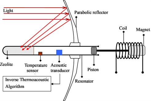
A self-excited thermoacoustic engine to harvest solar power is designed as in Fig. 4. It is assembled by the porous media, the acoustic resonator, the sunlight collector, and the mechatronic load. The thermoacoustic dynamics inside such a thermoacoustic engine can be represented into a feedback-loop interconnected by the heat-transfer dynamics of the porous media and the acoustic dynamics of working gas. On the interface with the acoustic resonator, the porous media has the heat-transfer affected by the temperature fluctuation that is algebraically dependent on the acoustic pressure as well as the entropy fluctuation thereon. Meanwhile, the heatflux fluctuation from the porous media initiates acoustic velocity that excites the acoustic motions distributed in the chamber [1], and thus forms the feedback loop. Imposed on those mean-flow conditions which characterize large loop-gains, the thermoacoustic dynamics can become linearly unstable up to limit-cycling (nonlinear vibration), or even up to mean-flow buckling (turbulence, streaming, vortex, etc.). Such thermoacoustic instability can be utilized for fast-time propulsion in thermoacoustic engines, but should be suppressed in combustion chambers to avert a variety of combustion instabilities.
Fig. 4Measurement of the heat-flux out of porous media in a self-excited thermoacoustic engine with inverse thermoacoustic algorithm
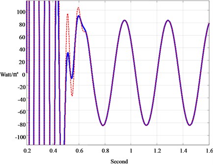
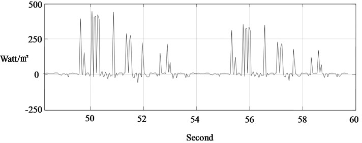
The ITAA developed in Section 3 is then employed to measure the heatflux out of the porous media, which is recorded in Fig. 5. It is found that PD-gradient rule catches the real heatflux with a phase lag, which is known from the measurement via PID-gradient rule. Fig. 6 is for the study on the sensitivity of converging times to P-gains in PID-adaptive observer. It shows that the converging time can be effectively shortened by enlargement of the P-gain. However, the converging time is unable to be arbitrarily small by adjusting the P-gain or D-gain, beyond some values of which the system exhibits in instability. Furthermore, the converging time is observed independent of the initial-state preset inside the PID-adaptive observer, as shown in the Fig. 7 wherein canonical responses of two initial-state guesses are plotted. This means that the sensor of entropy-flow can be turned on at any time, a necessary property for real-time operation.
Fig. 5Measurement of the porous-media heat-flux in Fig. 4 with PD and PID adaptive observers
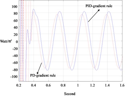
Fig. 6Converging times versus the P-gains of the PID-adaptive observer in heat-flux measurement of Fig. 4 (kD= 1000; kI= 100)
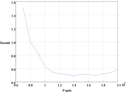
Fig. 5 demonstrates that the heatflux is of a sinusoidal shape, which verifies the limit-cycle oscillation. Furthermore, it is found by measurement that the entropy-flow across the interface between porous media and acoustic resonator is zero in average. That is, when the thermoacoustic process is fast-time drawing the internal energy in the thermal storage into vibration energy of fluid, the thermodynamics process is virtually isentropic. Therefore, the self-excited thermoacoustic engine is the most energy-efficient mechanism for converting heat to work, without considering the issue of power ratings. In the field of fluid fluctuation, it seems reasonable to assume that there is always some mechanism that can convert the internal energy into mechanical energy virtually without irreversibility, provided that the timescale of fluid fluctuation is short enough.
Fig. 7Responses with different guesses of initial state in the heat-flux measurement of Fig. 4 (kP= 10000; kI= 100; kD= 1000)
The second application is for measurement of impulsive heatflux. With the advent of thermally inductive materials [7], it becomes possible to design a thermal boost chopper as an electrical analogy to a step-up power converter. In the design, as shown in Fig. 8, Table 1, an electrically controlled micro-blind is chosen as the switching thermal-relay, and the thermally inductive material is to store and then to deliver heatflux along with the on-off of thermal relay in a cycle. According to the principle of boost choppers, the temperature drop from the thermal storage to the thermoacoustic transducer at their interface is impulsively large, by which a vigorous stream of heatflux will then be pumped into the thermoacoustic transducer at the frequency of thermal-relay switching. Fig. 9 shows the measured heatflux from the thermal storage to the thermoacoustic transducer. Even though the measured data are not clear enough to quantify the value of the thermal inductance, they are obviously impulsive. With such an impulsive heatflux, there is no doubt that thermal-inductance materials exist in nature.
Fig. 8Thermal boost chopper designed to study thermal inductance
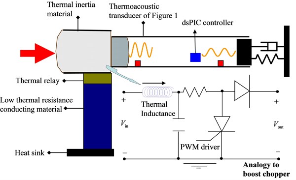
Table 1Thermal parameters measured at 25 degrees centigrade
Material | Thermal resistance (m∙K/W) | Thermal capacitance (J/m3∙k) | Thermal inductance (s∙m∙K/W) |
Agar | 1.646 | 4170451 | 6.01 |
Processed meat | 1.179 | 4069800 | 3.83 |
Sand | 0.8 | 1488960 | 1.24 |
NaHCO3 | 1.42 | 2246400 | 2.37 |
Fig. 9Measurement of thermal booster response with thermoacoustic transducer
5. Conclusion
Four tools are applied to design the thermoacoustic transducer for measurement of high-frequency or impulsive heatflux: (1) the heat-to-sound principle; (2) the virtual-source principle; (3) the structure of Luenberger observer; and (4) the PID-gradient rule (newly developed). This thermoacoustic transducer is then applied to verify the flowing two facts: (1) the isentropic process in the self-excited thermoacoustic instability; and (2) the existence of thermal inductance in nature.
References
-
Hong B.-S., Chou C.-Y. Energy transfer modelling of active thermoacoustic engines via Lagrangian thermoacoustic dynamics. Energy Conversion and Management, Vol. 84, 2014, p. 73-79.
-
Hong B.-S., Lin T.-Y. System identification and resonant control of thermoacoustic engines for robust solar power. Energies, Vol. 8, Issue 5, 2015, p. 4138-4159.
-
Hong B.-S., Wu M.-H. Online energy management of city cars with multi-objective LPV L2-gain control. Energies, Vol. 8, Issue 9, 2015, p. 9992-10016.
-
Beck J. V., Blackwell B., St Clair C. R. Jr. Inverse Heat Conduction: III-Posed Problems. John Wiley and Sons, New York, 1985.
-
Alifanov O. M. Inverse Heat Transfer Problems. Springer-Verlag, Heidelberg, 1994.
-
Jarny Y., Orlande H. R. B. Adjoint Methods in Thermal Measurements and Inverse Techniques. CRC Press, Boca Raton, 2011, p. 407-436.
-
Hong B.-S., Chou C.-Y. Realization of thermal inertia in frequency domain. Entropy, Vol. 16, 2014, p. 1101-1121.
-
Chou C.-Y., Hong B.-S., Chiang P.-J., Wang W.-T., Chen L.-K., Lee C.-Y. Distributed control of heat conduction in thermal inductive materials with 2D geometrical isomorphism. Entropy, Vol. 16, Issue 9, 2014, p. 4937-4959.
-
Feng Z. C., Chen J. K., Zhang Y. Real-time solution of heat conduction in a finite slab for inverse analysis. International Journal of Thermal Sciences, Vol. 49, 2012, p. 762-768.
-
Woodbury K. A., Beck J. V. Estimation metrics and optimal regularization in a Tikhonov digital filter for the inverse heat conduction problem. International Journal of Heat and Mass Transfer, Vol. 62, 2013, p. 31-39.
-
Woodbury K. A., Beck J. V., Najafi H. Filter solution of inverse heat conduction problem using measured temperature history as remote boundary condition. International Journal of Heat and Mass Transfer, Vol. 72, 2014, p. 139-147.
-
Najafi H., Woodbury K. A., Beck J. V. A filter-based solution for inverse heat conduction problems in multi-layer mediums. International Journal of Heat and Mass Transfer, Vol. 83, 2015, p. 710-720.
-
Najafi H., Woodbury K. A., Beck J. V., Keltner N. R. Real-time heat measurement using directional flame thermometer. Applied Thermal Engineering, Vol. 86, Issue 5, 2015, p. 229-237.
-
Ijaz U., Khambampati A., Kim M. C., Kim S. Estimation of time-dependent heatflux and measurement bias in two-dimensional inverse heat conduction problems. International Journal of Heat and Mass Transfer, Vol. 50, 2007, p. 4117-4130.
-
Kowsary F., Mohammadzaheri M., Irano S. Training based, moving digital filter method for real time heatflux function estimation. International Communications in Heat and Mass Transfer, Vol. 33, 2006, p. 1291-1296.
-
Hong B.-S., Su W.-J., Chou C.-Y. LPV modelling and game-theoretic control synthesis to design energy-motion regulators for electric scooters. Automatica, Vol. 50, Issue 4, 2014, p. 1196-1200.
-
Xiong Y., Saif M. Unknown disturbance inputs estimation based on a state functional observer design. Automatica, Vol. 39, 2003, p. 1389-1398.
-
Youssef T., Chadli M., Karimi H. R., Zelmat M. Design of unknown inputs proportional integral observers for TS fuzzy models. Neurocomputing, Vol. 123, 2014, p. 156-165.
-
Vijay P., Tade M. O., Ahmed K., Utikar R., Pareek V. Simultaneous estimation of states and inputs in a planar solid oxide fuel cell using nonlinear adaptive observer design. Journal of Power Sources, Vol. 248, 2014, p. 1218-1233.
-
Gao Z., Cecati C., Ding S. X. A survey of fault diagnosis and fault-tolerant techniques – Part 1: fault diagnosis with model-based and signal-based approaches. IEEE Transactions on Industrial Electronics, Vol. 62, Issue 6, 2015, p. 3757-3767.
About this article
