Sensor placement in the noise source identification based on acoustic radiation modes

Su, Jun-Bo; Zhu, Hai-Chao; Mao, Rong-Fu; Su, Chang-Wei; Guo, Liang

Vibroengineering Procedia

Browse Procedia

Published: 18 September 2015

Check for updates

Sensor placement in the noise source identification based on acoustic radiation modes

Jun-Bo Su¹

Hai-Chao Zhu²

Rong-Fu Mao³

Chang-Wei Su⁴

Liang Guo⁵

^{1, 2, 3, 4, 5}National Key Laboratory on Ship Vibration and Noise, Naval University of Engineering, Wuhan, China

Corresponding Author:

Hai-Chao Zhu

Cite the article Download PDF

Downloads 1137

Abstract

The noise source identification technology based on acoustic radiation modes could identify the noise source under less measuring points, while the sensor placement has great influence on the result of noise source identification. Under the prescribed number of sensors, a method to configure the measuring points is proposed. By the means of successive removal, select a set of measuring points in the candidate field points, which make the orthogonality of the acoustic field distribution modes matrix achieve the maximum value. The results of numerical simulation and sound box experiment have shown that when sensors are arranged in accordance with the measuring points selected by this method, the noise source could be identified effectively, and the identification result is better than that when sensors are arranged evenly.

1. Introduction

The near-field acoustic holography(NAH) proposed in the 1980s has obtained great success in noise source identification and localization, but the NAH requires a large number of sensors on the holographic plane, especially when applied to large structures. This limits NAH’s application in engineering practice. The acoustic radiation modes was proposed by Borgiotti etc. [1-3] in the 1980s, and have been applied in active structural acoustic control and sound power calculation [4, 5]. Jiang Zhe [6] and Nie Yong-Fa [7, 8] have proved that the acoustic radiation modes could be applied in the noise source identification with small amount of sensors. When the number of sensors is small, the arrangement method of sensors has important influence on the reconstruction result of surface’s velocities. If the sensor placement is illogicality, the reconstruction result would become worse due to the correlation between the data of sensors. A method to select measuring points in the acoustic field is proposed in this paper. The measuring points are selected from a set of candidate field points to make the vectors that comprise the acoustic field distribution modes matrix achieve the highest orthogonality. The effectiveness of the sensor placement method is verified by numerical simulation and sound box experiment.

2. Sensor placement in the noise source identification based on acoustic radiation modes

2.1. The theory of noise source identification based on acoustic radiation modes

The source’s surface can be decomposed a number of elements and the acoustic power radiated by the acoustic source may be written:

1

W = (\frac{s}{2}) R e [v^{H} Z v] = v^{H} R v,

in which $R = (s / 2) R e [Z]$ is the acoustic radiation resistance matrix; $Z$ is the acoustic radiation impedance matrix; $s$ is the area of the radiating element; $v$ is the vector of velocities on the source’s surface. Upon an eigen-decomposition of matrix, the matrix $R$ can be written as:

2

R = Φ Λ Φ^{H}

in which $Φ$ is an $N$ × $N$ orthogonal matrix including a acoustic radiation mode in each column. $Λ$ ( $Λ = d i a g [λ_{1}, λ_{2}, . . ., λ_{i}, . . .]$ ) is a diagonal matrix of which diagonal elements are the eigenvalues of $R$ . The vector of velocities on the source’s surface may be represented as:

3

v = Φ c,

in which $c$ is the expansion coefficient vector of acoustic radiation modes. Because the radiation efficiency of each acoustic radiation mode is proportional to the corresponding eigenvalue, the acoustic radiation modes are arranged in the matrix $Φ$ as the order of radiation efficiencies from high to low. Therefore vector of velocities on the source’s surface can be represented by the front parts of acoustic radiation modes. Assuming that the cutoff order number of acoustic radiation modes is $N_{1}$ , Eq. (3) becomes:

4

v \approx Φ_{1} c_{1},

in which $Φ_{1}$ is a $N$ × $N_{1}$ matrix; $c_{1}$ is a $N_{1}$ × $1$ vector.

In the acoustic near-field, M field points are selected to measure acoustic pressures. The vector of the pressures of the $M$ field points can be presented by acoustic radiation modes [8]:

5

P = j ρ c_{0} k G Φ_{1} c_{1},

in which $ρ$ is fluid density; $c_{0}$ is the sound speed in the fluid; $k$ is the wave number; $G$ is a $M$ × $N_{1}$ matrix whose elements are $G_{i j} = e^{- j k r_{i j}} / 4 π r_{i j}$ , $r_{i j}$ is the distance between the field point and the point on the source’s surface. Let $ψ = j ρ c_{0} k G Φ_{1}$ , the Eq. (5) becomes:

6

P = ψ c_{1} .

We define the column vectors of $ψ$ as the acoustic field distribution modes. The expansion coefficients of acoustic radiation modes $c_{1}$ can be solved by Eq. (6), then the vector of velocities on the source’s surface can be calculated by Eq. (4). The noise sources could be identified by the reconstructed velocities finally.

2.2. Sensor placement

Because the location of the sensors impacts the selection of the vectors that constitute acoustic field distribution modes matrix, the sensor placement has great influence on the solution of expansion coefficients of acoustic radiation modes. If the sensor placement is illogicality, the column vectors of the acoustic field distribution modes matrix may have high correlation property that make the condition number of the acoustic field distribution modes matrix too large. Large condition number would make the reconstruction result worse, due to the error produced in the process of solving expansion coefficients of acoustic radiation modes. Therefore, in this paper, the measuring points are selected by the criterion achieving the highest possible orthogonality property of the vectors that constitute acoustic field distribution modes matrix.

The same as Section 2.1, there are $M$ field points in the acoustic field, and the $M_{1}$ points of them are selected to solve the expansion coefficients. To make the equations well posed, we should select parts of the acoustic radiation modes. Assuming the cutoff order number of the acoustic radiation modes is $N_{1}$ ( $M_{1} > N_{1}$ ), the vector of the pressures of the $M$ field points can be reconstructed:

7

{p_{r}}_{(M \times 1)} = ψ_{(M \times N_{1})} {c_{1}}_{(N_{1} \times 1)} = ψ ψ^{+} {p_{0}}_{(M \times 1)} = U S V^{H} V S^{+} U^{H} {p_{0}}_{(M \times 1)} = U S S^{+} U^{H} {p_{0}}_{(M \times 1)} .

Eq. (7) shows that the reconstructed pressure vector is reconstructed by itself, so the matrix $T$ ( $T = U S S^{+} U^{H}$ ) must be a unit matrix. The diagonal elements of matrix $T$ and the elements of the reconstructed pressure vector are one-to-one correspondence. In order to eliminate the field point that is the most correlative to the smallest singular value, the last diagonal element of matrix $S$ and matrix $S^{+}$ in Eq. (7) are replaced by zero. Then the matrix $T$ is recalculated, and the field point that corresponds with the smallest diagonal element of the matrix $T$ is the most correlative to the smallest singular value. Therefore, an iterative process could be established for selecting the optimum sensor placement for a prescribed number of field points from a set of candidate points. Within each iteration, the matrix $T$ is calculated, and the field point that corresponds to the smallest diagonal value is eliminated from the set of candidate points. For the remaining points the matrices $U$ , $V$ and $S$ are evaluated again, and the product $T$ is computed. The elimination process continues until the number of the remaining field points is equal to the prescribed number. The whole iteration process would ensure that the condition number of the final acoustic field distribution modes matrix is the smallest.

3. Numerical simulation

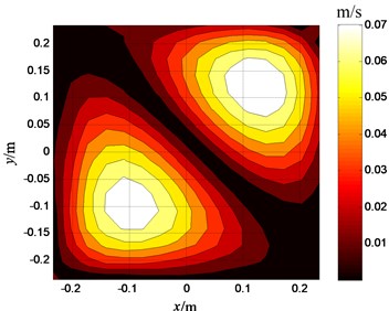
The validity of the proposed method in this paper is certified by a numerical simulation of a plate with infinite baffle. A single point-driven steel plate is selected, the dimensions of the plate are 0.5 m×0.5 m×0.008 m. The baffled plate is modeled in air with 16×16 constant boundary elements, and speed of sound of 340 m/s is assumed for air. When the plate is motivated by an exciting force with a frequency of 380 Hz, an amplitude of 10 N, the vibration mode of the plate is (1, 2). Fig. 1 shows the given particle velocity pattern of the plate.

Fig. 1The amplitude of velocity of the plate at the exciting frequency of 380 Hz

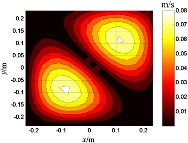
Fig. 2The optimal sensor placement

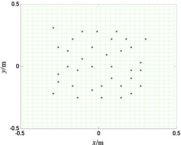
Fig. 3The even sensor placement

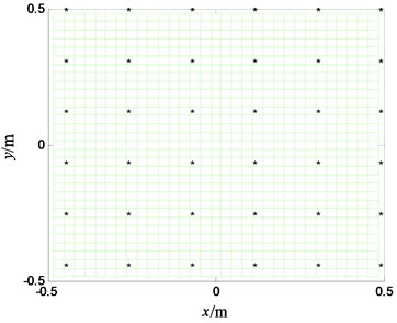
The measuring plane is placed in parallel with the plate in the acoustic field. The distance between the measuring plane and the plate is 0.1 m. The area of the measuring plane is four times of plate’s area, and there are 32×32 measuring points on the measuring plane. The theoretical values of measuring points are obtained by the Rayleigh integral. Supposing 36 measuring sensors are placed on the measuring plane, the sensor placement obtained by this paper’s method is shown as in Fig. 2. In addition, an even placement is selected for comparison which is as shown in Fig. 3.

The velocities on the plate surface are reconstructed respectively in the condition of the above two sensor placements. The reconstructed result by the sensor placement shown in Fig. 2 is shown in Fig. 4; the reconstructed result by the sensor placement shown in Fig. 3 is shown in Fig. 5. The reconstruction error of the first even placement is 3.2 %, the reconstruction error of the second even placement is 8.7 %. It can be seen from Fig. 4 that the two noise sources on the plate are identified accurately, and it can be known that the identification of the sensor placement selected by this paper is better than that of the even sensor placement from the comparison between Fig. 4 and Fig. 5.

Fig. 4Reconstructed velocities on plate’s surface (the optimal sensor placement)

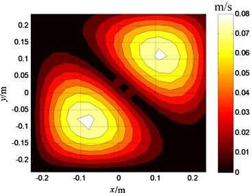
Fig. 5Reconstructed velocities of plate’s surface (the even sensor placement)

4. Sound box experiment

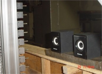
The sound box experiment is conducted in the open building. In this experiment, two sound boxes issue audio signals with the frequency of 100 Hz. The distance between the two sound boxes is 12 cm. The size of the measuring plane is 60 cm×50 cm. The measuring points is 13×11. The distance between two adjacent measuring points is 5 cm in both two directions. The distance between the measuring plane and the plane of sound boxes is 10 cm. The experimental scene is shown as Fig. 6.

Fig. 6The scene of experiment

In the reconstructing process, the size of source’s plane is equal to that of measuring plane, and 42 measuring points are selected in all the 143 measuring points. Two senor placements are selected to reconstruct the velocities of source’s plane, one is selected by the paper’s method; the other is an even placement, as shown in Fig. 7 and Fig. 8.

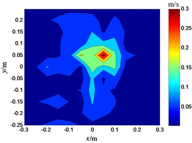
As shown in Fig. 9 and Fig. 10, the velocities of source’s plane are reconstructed by two sensor placement respectively. It can be seen from the two figures that the locations of two sound boxes are identified accurately in Fig. 9, while only one sound box’s location can be identified in the Fig. 10. That is to say, the reconstructed result of this paper’s sensor placement is better than that of the even sensor placement. The validity of the method for selecting the optimum sensor placement is verified by the experiment.

Fig. 7The optimal sensor placement on measuring plane

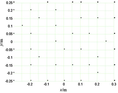
Fig. 8The even sensor placement on measuring plane

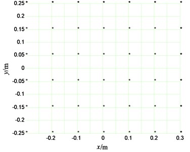
Fig. 9Reconstructed velocities of measuring plane (the optimal sensor placement)

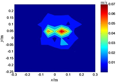
Fig. 10Reconstructed velocities of measuring plane (the even sensor placement)

5. Conclusions

A method to select the measuring points in the acoustic field is proposed to realize the noise source identification with small amount of sensors. The measuring points are selected from a set of candidate field points, which make the vectors that comprise the acoustic field distribution modes matrix achieve the highest orthogonality. The results of numerical simulation and sound box experiment have shown that when sensors are arranged in accordance with the measuring points selected by the proposed method, the noise source could be identified effectively, and the result is better than that when sensors are arranged evenly.

References

Borgiotti G. V. The power radiated by a vibrating body in an acoustic fluid and its determination from boundary measurements. The Journal of the Acoustical Society of America, Vol. 88, Issue 4, 1990, p. 1884-1893.

Search CrossRef
Cunefare K. A. The Design Sensitivity and Control of Acoustic Power Radiated by Three-Dimensional Structures. The Pennsylvania State University, 1990.

Search CrossRef
Elliott S. J., Johnson M. E. Radiation modes and the active control of sound power. The Journal of the Acoustical Society of America, Vol. 94, Issue 4, 1993, p. 2194-2204.

Search CrossRef
Peters H., Kessissoglou N. Enforcing reciprocity in numerical analysis of acoustic radiation modes and sound power evaluation. Journal of Computational Acoustics, Vol. 20, Issue 3, 2012, p. 5-33.

Search CrossRef
Wu Haijun, Jiang Weikang,Zhang Yilin A method to compute the radiated sound power based on mapped acoustic radiation modes. Journal of Computational Acoustics, Vol. 135, Issue 2, 2014, p. 679-692.

Search CrossRef
Jiang Zhe A modal analysis for the acoustic radiation problem: 1. Theory. ACTA Acustica, Vol. 29, Issue 4, 2004, p. 373-378.

Search CrossRef
Nie Yong-Fa, Zhu Hai-Chao Acoustic field reconstruction using source strength density acoustic radiation modes. ACTA Physica Sinica, Vol. 63, Issue 10, 2014, p. 104303.

Search CrossRef
Nie Yong-Fa, Zhu Hai-Chao The method of the identification of the planar noise source based on source strength acoustic radiation modes. Journal of Vibration Engineering, Vol. 27, Issue 4, 2014, p. 539-547.

Search CrossRef

About this article

Received

Accepted

31 August 2015

Published

18 September 2015

SUBJECTS

Fault diagnosis based on vibration signal analysis

Keywords

sensor placement

noise source identification

acoustic radiation modes

This is an open access article distributed under the Creative Commons Attribution License, which permits unrestricted use, distribution, and reproduction in any medium, provided the original work is properly cited.