Rolling bearing fault diagnosis by a novel fruit fly optimization algorithm optimized support vector machine

Chu, Dongliang; He, Qing; Mao, Xinhua

Journal of Vibroengineering

Browse Journal

Submit article

Published: 15 February 2016

Check for updates

Rolling bearing fault diagnosis by a novel fruit fly optimization algorithm optimized support vector machine

Dongliang Chu¹

Qing He²

Xinhua Mao³

^{1, 2, 3}School of Energy Power and Mechanical Engineering, North China Electric Power University, Beijing 102206, P. R. China

Corresponding Author:

Dongliang Chu

Cite the article Download PDF

Downloads 1227

WoS Core Citations 12

Abstract

Based on the nonlinear and non-stationary characteristics of rotating machinery vibration, a FOA-SVM model is established by Fruit Fly Optimization Algorithm (FOA) and combining the Support Vector Machine (SVM) to realize the optimization of the SVM parameters. The mechanism of this model is imitating the foraging behavior of fruit flies. The smell concentration judgment value of the forage is used as the parameter to construct a proper fitness function in order to search the optimal SVM parameters. The FOA algorithm is proved to be convergence fast and accurately with global searching ability by optimizing the analog signal of rotating machinery fault. In order to improve the classification accuracy rate, built FOA-SVM model, and then to extract feature value for training and testing, so that it can recognize the fault rolling bearing and the degree of it. Analyze and diagnose actual signals, it prove the validity of the method, and the improved method had a good prospect for its application in rolling bearing diagnosis.

1. Introduction

The key of fault diagnosis is the property of fault classifier, which should be with excellent robustness and generalization ability [1-3]. Among the research about mechanical fault diagnosis, the extensive used intelligent diagnosis methods are the neural network and expert system. On one hand, the neural network method is a heuristic method which mainly depends on experience. Its principle is the minimum of the experiential risk. This method lacks of solid theory foundation and is easy to occur the over-fitting phenomenon when the sample number is small. Besides, another deficiency of the neural network method is liable to be caught in local minimum. On the other hand, it is more necessary for the expert system method to establish perfect sample knowledge base. This method is lack of fault-tolerant ability. Moreover, it’s impossible to have enough fault sample in the practice which also limit the development of intelligent diagnosis system.

Differently, the support vector machine (SVM) method proposed by V. Vapnik is based on the statistical learning theory [4]. Its principle is the minimum of structural risk and takes account of training error and generalization ability. Therefore, this method is able to overcome local extremum, over-fitting and owe-fitting problem as well as small sample fitting problem [5, 6]. This method has been successfully applied in the function approximation, pattern recognition, regression analysis and signal processing field [7, 8]. What’s more, the classification accuracy will be significantly improved by optimizing the parameters of SVM.

At present, the commonly used parameter optimization algorithm include Grid Search (GS), Genetic Algorithm (GA) and Particle Swarm Optimization (PSO). GS algorithm tries to multiple zoom the range of parameters repetitiously relying on the experience to obtain the optimal solution which needs long time. GA and PSO algorithm both have many parameters and each parameter will directly influence the classification accuracy of SVM. Recently, Pan [9] proposed a new global optimization algorithm according to the foraging behavior of fruit fly, i.e. Fruit Fly Optimization Algorithm (FOA). Comparing with other group intelligent algorithms, the algorithm structure of FOA is simple and is understood conveniently. Its procedure code is easy to realize and needs less time. Moreover, this method has the ability of searching space and shows good characteristics of convergence and robustness [10-16]. In the present study, FOA algorithm is used to optimal the parameters of SVM by being inserted to the FOA-SVM model. The availability and accuracy of this method will be accessed by the simulation results that apply it in rolling bearing fault diagnosis.

2. Algorithm principle and modeling

2.1. Fundamental of FOA

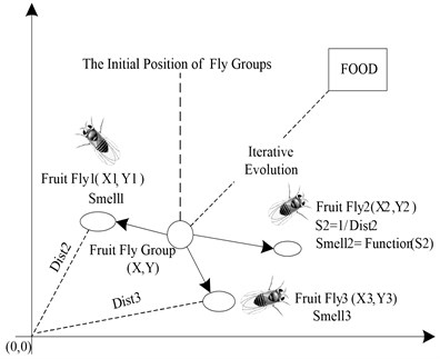
FOA algorithm is an optimizing method with good overall situation property, which is proposed through imitating the foraging process of fruit fly [9, 10]. It mainly rely on the acute olfactory of the fruit fly on the smell of forage. For fruit fly, the smell of the forage is related to the distance between the fruit fly and forage. It means that the smell of the forage decreased with the increment of the distance. Therefore, the process of foraging is the process of repeatedly moving from sites with mild smell to sites with strong smell. As shown in Fig. 1, the fruit flies with number of n firstly fly out to randomly direction from the original site. Then all these fruit flies will move to the site where one of the fruit fly stay who faces the strongest smell than other flies. In this way, a new position with fruit fly group is formed. This process of randomly fly out and gather again will be repeated again and again until the correct position of the forage is finally found out [15, 16].

Fig. 1Food finding iterative process of fruit fly swarm

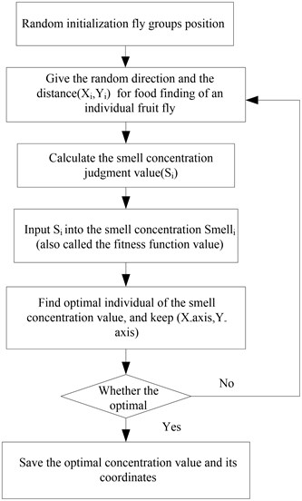
Similar with other algorithm, FOA is of some randomness during the process of the optimization. Therefore, in order to guide the right direction of fruit fly accurately, the smell concentration decision value and decision function are introduced into FOA which is similar with the fitness function in other evolutionary algorithm. The detail process is shown in Fig. 2.

The process of foraging of fruit fly can be formulated in the following necessary steps according to its habit [17, 18]:

Step 1: The original site of the fruit fly group is set down randomly, marked as coordinate ( $X$ , $Y$ ).

Step 2: Random direction and distance are given to the different fruit fly for foraging. The detail random distance is chosen by the position of original coordinate:

X_{i} = X + R a n d o m, Y_{i} = Y + R a n d o m .

Step 3: The distances between the position of fruit flies and the origin of coordinates are estimated as $D i s t_{i}$ . The reciprocal of the distances are set as the smell concentration decision value of fruit flies $S_{i}$ :

1

D i s t_{i} = \sqrt{X_{i}^{2} + Y_{i}^{2}}, S_{i} = \frac{1}{D i s t_{i}} .

Step 4: Put the smell concentration decision value of fruit flies $S_{i}$ into the smell concentration decision function (or called fitness function). The smell concentration of the individual fruit fly $S m e l l_{i}$ is obtained as:

S m e l l_{i} = F i t n e s s (S_{i}) .

Step 5: According to the initial smell concentration value of fruit fly, the extremum of the smell concentration among the fruit fly group is found out (the optimal individual):

[b e s t S m e l l b e s t I n d e x] = m a x (S m e l l_{i}) or [b e s t S m e l l b e s t I n d e x] = m i n (S m e l l_{i}) .

Step 6: The optimal gathering smell concentration of fruit fly is searched by smell. This concentration and the position of the fruit fly are recorded and saved as the optimal smell concentration $b e s t S m e l l$ and the present coordinate ( $X$ , $Y$ ), respectively:

2

X_{i} = X (b e s t I n d e x), Y_{i} = Y (b e s t I n d e x), S m e l l b e s t = b e s t S m e l l .

Step 7: The iterative optimization then starts by repeating the step 2 to 5. Under the precondition that the iterative number is smaller than the setting maximum iterative number, if the decision smell concentration is better than the previous iterative smell concentration, then step 6 should be carried out.

Fig. 2Flowchart of FOA

2.2. Fundamental of SVM

The basic idea of SVM is to obtain the special vector quantity by nonlinear mapping function. The special vector quantity satisfy that it bases on multi-dimensional sample input and one-dimensional sample output. Then the special vector quantity is used as input vector quantity to be mapped from the original space to high-dimensional characteristic space $H$ . Furthermore, an optimizing hyperplane is established in $H$ . That is [5]:

3

ω ϕ (x) + b = 0,

where $ω$ is weight vector, $b$ is threshold value.

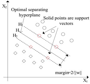
The two types of samples should be classified correctly by this hyperplane. Meanwhile, the hyperplane should satisfy the following constraint condition:

4

y_{i} [ω ϕ (x) + b] \geq 1, i = 1, 2, 3, \dots, l .

Only in this way, the hyperplane with maximal class interval can be obtained, that is the optimal classification plane, as shown in Fig. 3.

Fig. 3Optimal separating hyperplane (SVM)

The nonnegative slack variable $ξ$ , penalty factor $C$ and Lagrange multiplier $a_{i}$ were introduced to constraint optimization problem to the following problem:

5

\{\begin{array}{l} m a x H (a) = \sum_{i - 1}^{N} a_{i} - \frac{1}{2} \sum_{i = 1}^{N} \sum_{i = 1}^{n} y_{i} y_{j} a_{i} a_{j} ϕ (x_{i}) ϕ (x_{j}), \\ s . t . 0 \leq a_{i} \leq C, \sum_{i = 1}^{l} y_{i} a_{i} = 0 . \end{array}

According to KKT condition [6], the optimizing parameters should meet the following condition:

6

a_{i} \{y_{i} [ω ϕ (x) i + b] - 1 + ξ_{i}\} = 0 .

Finally, the optimal classification function can be obtained by solving the abovementioned problem, that is:

7

f (x) = s g n \{\sum_{i = 1}^{N} y_{i} a_{i} σ (x, x_{i}) + b\},

where $N$ is the number of support vector quantity and $σ (x, x_{i})$ is the kernel function.

The fitness function is:

8

f (σ^{2}, C) = \frac{1}{R (σ^{2}, C)},

where $R (σ^{2}, C)$ is the root mean square error of the training samples:

9

R = \sqrt{\frac{1}{n} \sum_{k = 1}^{n} e_{k}^{2}} .

In summary, penalty factor $C$ and kernel function parameter $σ$ are the key parameters that influence the performance of SVM classifier. Therefore, ( $C$ , $σ$ ) is used as the optimize variable in the present research.

2.3. FOA-SVM model

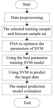
The FOA-SVM model is established by MATLAB program, as shown in Fig. 4. The necessary steps of establishing this model can be formulated as follow [19, 20].

Fig. 4FOA-SVM training steps

Step 1: The number of fruit fly group is set as Sizepop, and the number of iteration is set as Maxgen. As there are two parameters need to be optimized, the initial position of fruit fly ( $X$ , $Y$ ) should choose two random number for $X$ and $Y$ , respectively. Give the fly direction and distance of foraging for each individual fruit fly to get the initial coordinates ( $X_{1}$ , $Y_{1}$ ) and ( $X_{2}$ , $Y_{2}$ ). The distances between the individual fruit fly and the origin of coordinates are estimated as the smell concentration decision value $S_{1 i}$ and $S_{2 i}$ .

Step 2: Choose the appropriate decision value to determine the range of penalty factor $C$ and kernel function parameter $σ$ : $C = m S_{1 i}$ , $σ = n S_{2 i}$ . And then modify the value of $m$ and $n$ according to the range of $C$ and $σ$ . In this study, the range of $C$ and $σ$ are $C \in [0, 1000]$ and $σ \in [0, 100]$ . In order to limit the domain of definition of $S$ located in [0, 10], the value of m and n are choose as $m =$ 100 and $n =$ 10.

Step 3: Training the data base characteristic value by SVM model and get the fitness function.

Step 4: The highest smell concentration of fruit fly is the maximum of fitness. Save the coordinate of this fruit fly and set it as the initial optimal coordinate.

Step 5: The iterative optimization starts. The optimal fitness function and the values of $C$ and $σ$ are saved. Attention that the optimal fitness corresponding with many $C$ and $σ$ values. When value of $C$ is oversize, the error will be increased. Therefore, the minimum value of $C$ and the corresponding $σ$ should be saved.

3. Analysis of simulation signal

The investigated signal is shown as follow [21]:

10

x (t) = 2 s i n 2 π f_{1} t + 1.5 s i n 2 π f_{2} t + 15 e^{- \frac{(t - 300)^{2}}{2}} s i n 200 t .

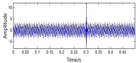
This simulation signal imitates the short time shock when the fault of the rotating machinery occurs. It is the superposition of a nonlinear signal and two sine signals. The sampling frequency is 2048 Hz while the sample number is 1024 points. The signal frequency is $f_{1} =$ 200 Hz and $f_{2} =$ 200 Hz. The time-domain plot of the imitation signal is shown in Fig. 5. As shown in Fig. 5, the amplitude changes sharply at 0.3 s. It indicates that the rotating machinery is facing the shock [22].

Fig. 5Analog signal time domain waveform figure

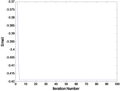
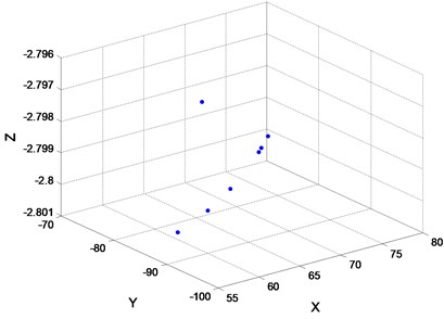
After times of attempt, the number of fruit fly is set as 20. The iterative number is 100 times. The initial position section is [0, 10]. The searching direction and distance section is [–1, 1]. The finally convergence extremum after FOA global optimization is quite close to –3.418 (Fig. 6(a)). The calculating time is 1.24 s. Fig. 6(b) is the fly track of fruit fly when optimizing.

Fig. 6a) 100 iterations of FOA global optimization curve; b) FOA route search trajectory

a)

b)

Thus, these data suggest that the relatively small amount of calculation of fruit fly optimization algorithm. A period of time from the beginning, it doesn’t appear that independent variables are continuous oscillation. Finally, the global optimization converge to the signal of the extremum. The results show that the optimization precision is very high.

4. Experimental validation

To illustrate the proposed intelligent diagnosing method, the fault diagnosis of rolling element bearings is studied by using real data obtained from experiment and engineering application, respectively.

4.1. Fault diagnosis process of rolling bearing

The detail method is shown in Fig. 7. The vibration signal of rolling bearing is pretreated by ensemble empirical mode decomposition (EEMD) to obtain the kurtosis of all the component of Intrinsic Mode Function (IMF). Then the obtained kurtosis and the original signal kurtosis are made up of characteristic vectors. The work state and the fault type are then identified using SVM as the classifier [23-27].

Fig. 7The flow chart of fault diagnosis

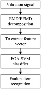
Firstly, sample the four types of fault of rolling bearing with a certain sampling frequency. The four types of faults are recognized as normal fault, inner ring fault, outer ring fault and rolling element fault.

Secondly, EEMD resolving is used to every sample signal to obtain the of IMF component of each signal.

Thirdly, obtain the kurtosis of each signal and its IMF component to make up of the characteristic vector quantity.

Fourthly, input half of the characteristic vector quantity of the four state of antifriction bearing into SVM and train it.

Finally, a half of the characteristic vectors are used as testing sample to calculate separately. The output results of classification function are then compared with the true fault type (or working state) of the testing samples to obtain the correct rate.

4.2. Data introduction

The data used for testing the efficiency of the proposed method in this research comes from the data center of Case Western Reserve University, USA [28]. The testing platform contains driving motor, torque sensor, ergometer and electric control device. The drive end of the motor shaft is supported by the JEMSKF6025-2RS deep groove ball bearing with fault. The geometry parameters of the bearing are shown in Table 1.

Single point fault is put on the inner ring, outer ring and rolling element. The sampling frequency is 12000 Hz. The data of the four fault types, i.e. normal, inner ring, outer ring and rolling element fault, is shown in Table 2. The different pitting diameters reflect the different level of fault. In detail, 7 inch means that the fault is early failure or mild failure while 28 inch means major failure. All the data are divided into 8 groups for ensemble empirical mode decomposition according to the working state and fault level. Furthermore, the kurtosis of the rolling bearing is calculated and the groups of the characteristic vectors are obtained.

Table 1Rolling bearing information size (mm)

Type	Diameter		Thickness	Pitch diameter
	Outer	Inner
SKF6205-2RS	25	52	15	39

Table 2Data distribution instructions of the experimental bearing

Status	Labels	Pitting diameter (inch)	Data code
Normal	1	0	97	98	99	100
Inner ring fault	2	7	105	106	107	108
	3	14	169	170	171	172
	4	21	209	210	211	212
	5	28	3001	3002	3003	3004
Outer ring fault	6	7	144	145	146	147
Outer ring fault	7	21	246	247	248	249
Rolling element fault	8	7	118	119	120	121

Before input the data into SVM classifier, a certain amount of the characteristic vector quantity group is chosen as the sample set. Among this, category 1 (normal fault) owns 80 groups of data while the other 7 categories own 40 groups respectively. Besides, for each category, half of the data is used as training sample while the other half of the data is used as testing sample.

4.3. Results analysis

The evolutionary iterative process of searching for the optimal parameters for experimental bearing using FOA is shown in Fig. 8 and Fig. 10. For the determination of parameters in FOA algorithm, the initial fruit fly group setting section is [0, 1]. The size of the group is 20. The number of the iterative is 100.

Fig. 8FOA fitness of finding the best parameters of the graph for experimental bearing (EMD)

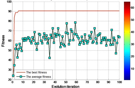
By the EMD decomposition test samples, the results of FOA searching show that the optimal $C =$ 64.6741 and optimal $g =$ 0.38582 (Fig. 8). However, the accuracy of the fault diagnosis is 90.5556 %. By the EEMD decomposition test samples, the results of FOA searching show that the optimal $C =$ 91.4004 and optimal $g =$ 0.083933 (Fig. 10). More importantly, the accuracy of the fault diagnosis is higher than 95 %.

According to data comparison of the figure, test sample of EEMD decomposition fault diagnosis through the FOA-SVM, significantly higher than that of the EMD decomposition of test samples.

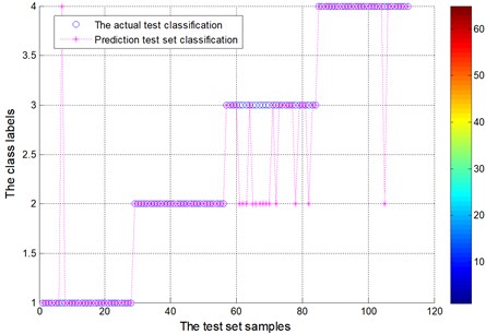
Fig. 9Test set of the actual classification and prediction classification figure for experimental bearing (EMD)

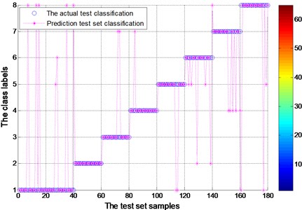
Fig. 10FOA fitness of finding the best parameters of the graph for experimental bearing (EEMD)

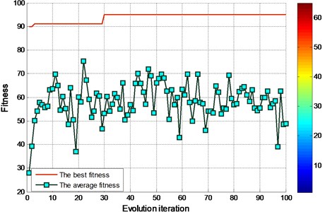
Fig. 11Test set of the actual classification and prediction classification figure for experimental bearing (EEMD)

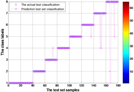
As shown in Fig. 9 and Fig. 11, the hollow circle represents the actual test classification label while the star represents the predicted classification results through SVM classifier. The abscissa is the 180 testing samples while the ordinate represents the 8 categories. Each category contains 20 samples except the category 1 which contains 40 samples. The EMD and EEMD test sample actual classification accuracy, is shown in Table 3. It has the overall accuracy and the accuracy of all kinds of the label. Fault feature of vibration signal by EEMD decomposition as a result of actual classification is obviously better than that of the EMD decomposition results. As the same time, test sample of EEMD decomposition fault diagnosis through the FOA-SVM, significantly higher than that of the EMD decomposition of test samples. It is obvious that the predicted results fit the actual fault very well. In particularly, the rotating element fault can also be distinguished correctly. Therefore, the FOA-SVM is proved to have good property and can solve the problem of lacking of samples in the practice. What’s more, according to different samples, FOA-SVM fault diagnosis is more accurate and more reliable.

Table 3Actual classification results of experimental bearing

Label	Accuracy (%) EMD	Accuracy (%) EEMD
Label	$C =$ 64.674, $g =$ 0.38582	$C =$ 91.4004, $g =$ 0.083933
Whole	85.5556	96.1111
1	82.5	100
2	100	100
3	90	95
4	95	100
5	90	100
6	70	95
7	75	90
8	85	85

5. Engineering application

To further verify the classification performance of FOA-SVM, in the section, the proposed method is applied to bearing fault diagnosis for electric locomotives. Diagnosis of electric locomotive roller bearings is of great significance in industry.

5.1. Data introduction

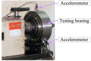
Fig. 12 shows the test bench of a locomotive roller bearing. The bench consists of a hydraulic motor, two supporting pillow blocks. The bearing is installed in a hydraulic motor driven mechanical system. Accelerometers are mounted on the load module adjacent to the outer race of the test bearing for measuring its vibration.

Fig. 12Test bench of a locomotive roller bearing

A bearing data set containing four subsets is normal, inner ring, outer ring and roller element fault. The four conditions are described in Table 4. Three fault cases of locomotive roller bearings are shown in Fig. 13. Fig. 14 gives raw data samples for the four bearing conditions. Among this, all categories own 32 groups of data respectively. Besides, for each category, half of the data is used as training sample while the other half of the data is used as testing sample.

Fig. 13Faults in the locomotive roller bearings

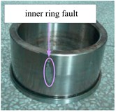
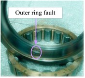
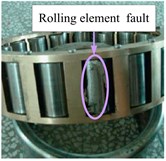
Table 4Data distribution instructions of the locomotive bearing

Status	Rotating speed (r/min)	Label
Normal	490	1
Inner ring fault	480	2
Outer ring fault	500	3
Rolling element fault	530	4

5.2. Results analysis

The evolutionary iterative process of searching for the optimal parameters for locomotive bearing using FOA is shown in Fig. 14 and Fig. 16.

Fig. 14Test set of the actual classification and prediction classification figure for locomotive bearing (EMD)

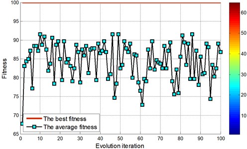
Fig. 15Test set of the actual classification and prediction classification figure for locomotive bearing (EMD)

By the EMD decomposition test samples, the results of FOA searching show that the optimal $C =$ 10.4135 and optimal $g =$ 0.01 (Fig. 14). However, by the EEMD decomposition test samples, the results of FOA searching show that the optimal $C =$ 0.1 and optimal $g =$ 0.01.

According to data comparison of the figure, test sample of EEMD decomposition fault diagnosis through the FOA-SVM, significantly higher than that of the EMD decomposition of test samples.

Fig. 15 and Fig. 17 show test set of the actual and prediction classification for locomotive bearing. In the locomotive bearing case, fault feature of vibration signal by EEMD decomposition as a result of actual classification is obviously better than that of the EMD decomposition results. Table 5 gives the testing accuracies of the two methods are 87.5 % and 98.2143 %, respectively. Compared with the average accuracy of EMD decomposition fault diagnosis, EEMD decomposition method increases the recognition accuracy about 10 %. Therefore, the locomotive testing results further verified that FOA-SVM can reliably separate different fault conditions.

Fig. 16Test set of the actual classification and prediction classification figure for locomotive bearing (EMD)

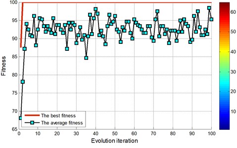
Fig. 17Test set of the actual classification and prediction classification figure for locomotive bearing (EEMD)

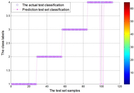
Table 5Actual classification results of experimental bearings

Label	Accuracy (%) EMD	Accuracy (%) EEMD
Label	$C =$ 10.4135, $g =$ 0.01	$C =$ 0.1, $g =$ 0.01
Whole	87.5	98.2143
1	96.4286	100
2	100	100
3	57.1429	100
4	96.4286	92.8571

The authors declare that there is no conflict of interests regarding the publication of this paper.

6. Conclusions

The experiment results demonstrated that WSVM is effective in handling uncertain data and small samples. Moreover, it is shown that PSO presented here is effective for the WSVM (or SVM) to seek optimized parameters.

A new fault diagnosis method based on FOA and SVM is proposed in the present study. The different fault of inner ring, outer ring and rotating element are efficiently distinguished by the established FOA-SVM model. The experiment and engineering application results demonstrated that FOA is effective in handling uncertain data and small samples. In particular, test sample of EEMD decomposition fault diagnosis through the FOA-SVM, the effect is more accurate. The choice about step size parameter of FOA directly affects its execution efficiency and accuracy, therefore, when solving practical problems, how to select suitable step length automatically, that need to be further in-depth study.

References

Peng Zhingke, He Yongyong, Lu Qing, et al. Using wavelet method to analysis fault features of rub rotor in generator. Proceedings of the CSEE, Vol. 23, Issue 5, 2003, p. 75-79, (in Chinese).

Search CrossRef
Zhang Jun, Han Pu, Dong Ze, et al. Energy leakage research of wavelet transform application on vibration signature analysis. Proceedings of the CSEE, Vol. 24, Issue 10, 2004, p. 238-243, (in Chinese).

Search CrossRef
Hong Ye, Li Guohong, Cai Weiyou, et al. Fault diagnosis of hydro-generator unit vibration based on wavelet packet analysis. Engineering Journal of Wuhan University, Vol. 35, Issue 1, 2002, p. 65-68, (in Chinese).

Search CrossRef
Vapnik V. N. The Nature of Statistical Learning Theory. Springer-Verlag, New York, 1995.

Search CrossRef
Ding Shifei, Qi Bingjuan, Tan Hongyan An overview on theory and algorithm of support vector machines. Journal of University of Electronic Science and Technology, 2011, p. 2-10.

Search CrossRef
Wu Chongming, Wang Xiaodan, Bai Dongying, et al. Fast SVM incremental learning algorithm using KKT conditions and between-class convex hull vectors. Computer Engineering and Design, Vol. 31, Issue 8, 2010, p. 1792-1795, (in Chinese).

Search CrossRef
Poyhonen S., Negrea M., Arkkio A., Hyotyniemi H., Koivo H. Fault diagnostics of an electrical machine with multiple support vector classifiers. Proceedings of IEEE Interactional Symposium on Intelligent Control, Vancouver, 2002.

Search CrossRef
Hsu Chihwei, Lin Chihjen A comparison of methods for multi-class support vector machines. IEEE Transactions on Neural Networks, Vol. 13, Issue 2, 2002, p. 415-425.

Search CrossRef
Pan W. T. Fruit Fly Optimization Algorithm. Tsang Hai Book Publishing Co., Taipei, China, 2011, p. 10-11, (in Chinese).

Search CrossRef
Hu Neng-fa Evolutionary fruit algorithm and its application research. Computer Technology and Development, Vol. 7, 2013, p. 131-133, (in Chinese).

Search CrossRef
Zhang Xiang, Chen Lin Fault diagnosis based on support vector machines optimized by fruit fly optimization algorithm. Electronic Design Engineering, Vol. 21, Issue 16, 2013, p. 90-93, (in Chinese).

Search CrossRef
Wang X., Zou Z. Identification of ship manoeuvring response model based on fruit fly optimization algorithm. Journal of Dalian Maritime University, Vol. 38, Issue 3, 2012, p. 1-5, (in Chinese).

Search CrossRef
Pan Q. K., Sang H. Y., Duan J. H., et al. An improved fruit fly optimization algorithm for continuous function optimization problems. Knowledge-Based Systems, Vol. 62, 2014, p. 69-83.

Search CrossRef
Pan W. T. A new fruit fly optimization algorithm: taking the financial distress model as an example. Knowledge-Based Systems (SCI), Vol. 29, 2012, p. 69-74.

Search CrossRef
Li H., Guo S., Zhao H., Su C., Wang B. Annual electric load forecasting by a least squares support vector machine with a fruit ﬂy optimization algorithm. Energies, Vol. 5, 2012, p. 4430-4445.

Search CrossRef
Li H.-Z., Guo S., Li C.-J., Sun J.-Q. A hybrid annual power load forecasting model based on generalized regression neural network with fruit ﬂy optimization algorithm. Knowledge-Based Systems, Vol. 37, 2013, p. 378-387.

Search CrossRef
Pan W.-T. Using fruit fly optimization algorithm optimized general regression neural network to construct the operating performance of enterprises model. Journal of Taiyuan University of Technology: Social Sciences Edition, Vol. 29, Issue 4, 2012, p. 1-5, (in Chinese).

Search CrossRef
Zhou J., Wang C., He B. Forecasting model via LSSVM with mixed kernel and FOA. Computer Engineering and Applications, Vol. 33, Issue 4, 2013, p. 964-966, (in Chinese).

Search CrossRef
Niu P., Ma H., Li G., et al. Study on No_x emission from CFB boilers based on support vector machine and fruit fly optimization algorithm. Journal of Chinese Society of Power Engineering, Vol. 33, Issue 4, 2013, p. 267-271, (in Chinese).

Search CrossRef
Wang X., Zou Z. FOA-Based SVM parameter optimization and its application in ship manoeuvring prediction. Journal of Shanghai Jiao Tong University, Vol. 6, 2013, p. 6, (in Chinese).

Search CrossRef
Wang Xuhui Research and Application of Fault Feature Extraction for Rotating Machinery. North China Electric Power University, Beijing, 2010, p. 41-42, (in Chinese).

Search CrossRef
Chen Junsheng, Zhang Kang, Yang Yu, et al. Comparison between the methods local mean decomposition and empirical mode decomposition. Journal of Vibration and Shock, Vol. 28, Issue 5, 2009, p. 13-16, (in Chinese).

Search CrossRef
Cheng J. S., Yu D. J., Yang Y. Roller bearing fault diagnosis method based on SVM and EMD envelope spectrum. Systems Engineering Theory and Practice, Vol. 25, Issue 9, 2006, p. 131-136, (in Chinese).

Search CrossRef
Wu Z., Huang N. E. Ensemble empirical mode decomposition: a noise-assisted data analysis method. Advances in Adaptive Data Analysis, Vol. 1, Issue 1, 2009, p. 1-41.

Search CrossRef
Pines D., Salvino L. Structural health monitoring using empirical mode decomposition and the Hilbert phase. Journal of Sound and Vibration, Issues 1-2, 2006, p. 97-124.

Search CrossRef
Zhang Chao, Chen Jian-jun, Xu Ya-lan A bearing fault diagnosis method based on EMD and difference spectrum theory of singular value. Journal of Vibration Engineering, Vol. 24, Issue 5, 2011, p. 539-545, (in Chinese).

Search CrossRef
Lei Y. G., Lin J., He Z. J., et al. Application of an improved kurtogram method for fault diagnosis of rolling element bearings. Mechanical Systems and Signal Processing, Vol. 25, 2011, p. 1738-1748.

Search CrossRef
The Case Western Reserve University Bearing Data Center [EB/OL]. http://csegroups.case.edu/hearingdatacenter/pages/download-data-file, 2012.

Search CrossRef

About this article

Received

18 August 2015

Accepted

10 December 2015

Published

15 February 2016

SUBJECTS

Fault diagnosis based on vibration signal analysis

Keywords

support vector machine

fruit fly optimization algorithm

parameter optimization

fitness function

fault diagnosis

rotating machinery vibration

Acknowledgements

This work is supported by the Fundamental Research Funds for the Central Universities (No. 14XS25).

This is an open access article distributed under the Creative Commons Attribution License, which permits unrestricted use, distribution, and reproduction in any medium, provided the original work is properly cited.