Abstract
This paper presents an investigation on modal simulation of turbocharger impeller with considering fluid-solid interaction. To demonstrate how the fluid-solid interaction affects modal parameters of the turbocharger impeller, a fluid field model of the impeller was established based on the theory of turbulence flow. Then the fluid grid was discretized and the fluid boundary condition was loaded. After obtaining the velocity and pressure distribution of the inner flow filed of the impeller by simulations, the distributed pressure was loaded onto the structure surface of the impeller to calculate the modal parameters of the impeller. Simulation results show that the solid-fluid coupling field has an influence mainly on the modal frequencies of the impeller, and less on its modal shapes. The simulation results are very useful for designing turbocharger impeller.
1. Introduction
While the turbocharger operates in high rotational speeds, its impeller is exposed to the high-speed flow of the gas field environment, which has a significant impact on the impeller’s performances and vibration characteristics. At the same time, the vibrations of the impeller’s structure in turn affect the flow field, thereby forming a fluid-structure interaction model. A thorough fluid-solid interaction vibration investigation was, however, very difficult and relatively few studies were published. Most researchers have attempted to discover the impact of the flow field on the turbocharger performance [1-5]. Some previous investigations employed the coupled CFD-FEM model to calculate the dynamic responses in rotating blades exposed to steady and unsteady aerodynamic forces [6-9]. Other previous studies employed the FEM model to calculate the blade modes without considering the aerodynamic forces [10-12].
The main research work of this paper is to establish the turbocharger compressor CFD model and the structure FEM model, and then form the fluid-structure interaction simulation model and demonstrate how the impact of high velocity gas affects the modal parameters of the turbocharger impeller.
2. CFD model and simulation
2.1. Turbulence model
The - turbulence model with scalable wall functions was employed. The turbulence viscosity coefficient in the algebraic turbulence model is determined by mixing length and has nothing to do with turbulent kinetic energy. But in the turbulent transport model, the turbulence viscosity coefficient is related to turbulent kinetic energy and other turbulent parameters [13, 14]. Under not considering the effect of gravities, the transport equations of standard - turbulent model can be expressed by:
where is the space coordinate of the actual flow area and is the turbulent kinetic energy, generated by the average velocity gradient, and:
In Eq. (3), both and are the average pulse velocities.
In Eq. (2), is the model parameter, and . , , , and are also model parameters. Their values are listed in Table 1 [15].
Table 1Parameters of standard κ-ε turbulent model
Parameters | |||||
Values | 0.09 | 1.00 | 1.30 | 1.44 | 1.92 |
2.2. Discretization
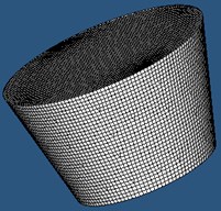
The entire flow field, which divided into three sections, respectively as the inlet flow area, impeller flow field area and the volute area, was discretized by using HYPERMESH [15]. The grid discretization is an important pre-treatment process. For the simulation of complex regions of the flow, heat transfer and other issues, the grid resolution directly affects the accuracy of calculation. During the grid discretization, the grid resolution is a compromise between expected results and numerical effort. High resolutions of boundary layers, very detailed secondary flows and very accurate captures of shocks cannot be expected with this mesh density. Table 2 shows the meshing details. Figs. 1-4 show the grids of impeller flow model, inlet flow model, volute flow model and the whole compressor flow model respectively.
Table 2Details of meshing for compressor
Grid description | Grid accuracy parameter | Impeller | Volute | Inlet |
Blocks of grid | 247133 | 519911 | 227133 | |
Total nodes | 70302 | 127834 | 70302 | |
Quality of grids | Warpage | 8.50 | 8.50 | 6.89 |
Aspect ratio | 61.44 | 5.00 | 51.78 | |
Skew angle | 85.34 | 60.10 | 64.58 | |
Jacobian | 0.63 | 0.65 | 0.65 |
Fig. 1The grids of impeller flow area
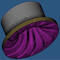
Fig. 2The grids of inlet flow area
2.3. Initial conditions and boundary conditions
The static pressure of the compressor volute outlet was used to adjust the rate of flow of the compressor. For a solid wall, taken as impermeable, there were no slip and adiabatic boundary conditions. As a result, the mass flux, momentum flux and energy flux which pass through the meshed surface coinciding with the solid boundary were zero. The interfaces ‘impeller/suction elbow’ and ‘impeller/vaneless diffuser’ have been treated as steady ‘rotor/stator’ interfaces. Therefore, for every time step a ‘frozen rotor interface’ or ‘mixing-plane interface’ was defined.
In the following simulation, RNG - model was utilized and air density was 1.225 kg/m3. The inlet condition of the compressor was set as Table 3.
The periodic boundary conditions were used for both walls of the one seventh of the compressor impeller channel, and the mixing planes were defined for impeller outlet and volute inlet. No slip and adiabatic boundary condition were defined for wall surface.
Fig. 3The grids of the volute area
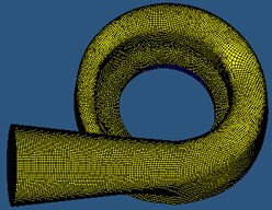
Fig. 4The grids of the whole compressor flow model
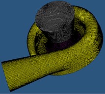
Table 3Inlet condition of compressor
No. | Rotating speed | Pressure | Temperature | Flow rate |
1 | 90,000 rpm | –2.1 kPa | 25.8 °C | 0.037820 kg/s |
2 | 110,000 rpm | –2.3 kPa | 25.5 °C | 0.049056 kg/s |
3 | 130,000 rpm | –2.5 kPa | 25.3 °C | 0.063056 kg/s |
2.4. Numerical procedure
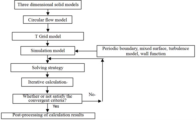
The numerical simulation procedure of the inner flow field of the compeller, by using CFD method, includes the following several steps: firstly beginning with its specific geometry boundary conditions and the physical boundary conditions, then numerically simulating the flow field under the basic controlling flow equations such as the mass conservation equation and momentum conservation equation to obtain a three-dimensional flow field distribution of the various basic physical quantities, and then do post-processing on the above data to get the interesting physical quantities, such as the flow velocity distribution and pressure distribution. The basic process is shown in Fig. 5.
Fig. 5Procedure of numerical simulation of flow-field
2.5. Settings for solver
In the simulation of the steady flow of turbocharger compressor, the SIMPLC algorithm was used for pressure correction. In order to overcome the false diffusion, the convection terms were dispersed by using the QUICK scheme with third-order accuracy, the diffusion source terms were dispersed by using the second-order central scheme, and the time terms were dispersed by using the second-order implicit format.
As the blades of the impeller uniformly distributed along the circumference and its rotating speed is considered as constant, so the relative motion between the impeller flow and the volute is periodic, and the time step of the compressor simulation is determined as follows:
where is the step number for the calculation period of the steady flow, and 20. is the rotating speed of the impeller. The time step is calculated with Eq. (4) and Table 4 shows its values [15-17].
Table 4Time step
Rotating speed | 80,000 rpm | 100,000 rpm | 120,000 rpm | 140,000 rpm |
Time step(s) | 6.25E-6 | 5.00E-6 | 4.167E-6 | 3.57E-6 |
2.6. Convergence judgment for simulation
1) Each block residual and the overall residual decrease by three orders of magnitude, compared with previous iteration.
2) The relative error of outlet flux and inlet flux are less than 0.5 % respectively.
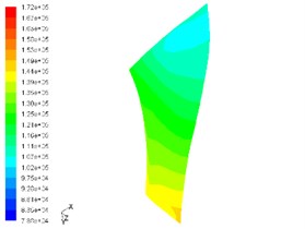
Fig. 6Static pressure contour on pressurized surface of main blade and shunt blade at speed of 110,000 rpm
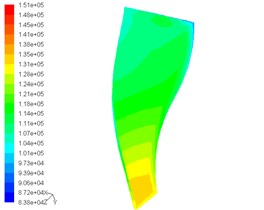
a) Pressure contour on pressurized side of main blade
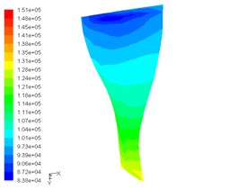
b) Pressure contour on suction side of main blade
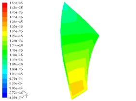
c) Pressure contour on pressurized side of shunt blade
d) Pressure contour on suction side of shunt blade
2.7. Centrifugal compressor flow analysis
According to the CFD simulation models and numerical simulation procedures for the internal flow of the turbocharger compressor, the CFD simulations was performed with FLUENT6.3 using a grid with 994,177 cells and the static pressure, velocity vectors of the compressor at different rotating speeds were obtained, shown as Fig. 6 to Fig. 10.
Fig. 7Static pressure contour on pressurized surface of main blade and shunt blade at speed of 130,000 rpm
a) Pressure contour on pressurized side of main blade
b) Pressure contour on suction side of main blade
c) Pressure contour on pressurized side of shunt blade
d) Pressure contour on suction side of shunt blade
Fig. 8Velocity vectors on blade surfaces
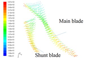
a) At speed of 110,000 rpm
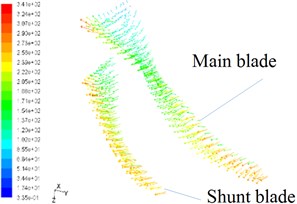
b) At speed of 130,000 rpm
Fig. 9Static pressure contour of non-leaf diffuser and volute surfaces
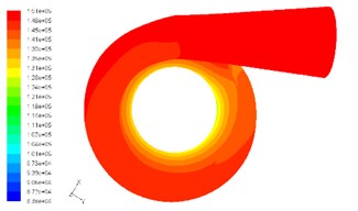
a) At speed of 110,000 rpm
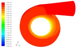
b) At speed of 130,000 rpm
According to the simulation data, the following phenomena could be observed:
1) The pressure gradient change on the suction side of blades is higher than on the pressurized side of blades and compared with the shunt blades, the pressure gradient of the main leaf blades is more obvious.
2) From the velocity vector maps, it could be found that the gas flow inside the impeller is relatively complex. When the air is inhaled into the impeller, the impeller drives the air rotating, and creates the gas flow rate to increase. Under the action of the gas centrifugal force, the gas is thrown to the edge of the impeller, but the flow change is relatively uniform. And because the channel between the blades is as fan-shaped expansion, and the relative speed of the flow air decreases, so the pressure at this channel increases.
Imported the turbulence computation, obtained by above flow-field simulation, the CFD-FEM model was employed to calculate the modal parameters of the impeller.
Fig. 10Velocity vectors of non-leaf diffuser and volute surfaces
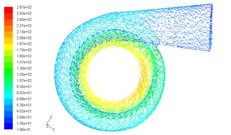
a) At speed of 110,000 rpm
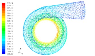
b) At speed of 130,000 rpm
3. Modal simulation of compeller with CFD-FEM model
3.1. FEM model of compressor impeller
Fig. 11(a) is the compressor impeller photo and the diameter of its hub is 78 mm. This impeller contains seven main blades and seven shunt blades totally. The three dimension model of this impeller has been established with UG software and was meshed by using HYPERMESH with a grid with 98,590 cells. The 3D solid model and FEM model are shown as Fig. 11(b) and Fig. 11(c) respectively.
Fig. 11FEM model of compressor impeller
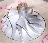
a) A photo
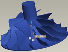
b) 3D solid model
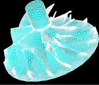
c) FEM model
3.2. CFD-FEM model of compressor impeller
The flow field data from above CFD simulation was imported by using ANSYS software interface. After the boundary conditions were defined appropriately, the pressures of fluid field were loaded onto the impeller surfaces and the calculation of CFD-FEM coupled field was performed. The boundary conditions are included as:
1) On interface surface between flow field and solid structure:
where is normal direction of immersed surface of solid structure, and is normal velocity of immersed surface of solid structure.
2) On solid interface :
3) On fluid interface.
Under low frequency condition, the boundary conditions were simplified as:
Under high frequency condition, and according to the equation , so can be obtained and the boundary conditions on free surfaces can be simplified as:
The fluid-solid coupled vibration equations of compressor impeller are shown as:
where , and are structural mass matrix, structural stiffness matrix and structural damping matrix respectively. is force vector at structural nodes. , and are fluid mass matrix, fluid stiffness matrix and fluid damping matrix respectively. is fluid density. is fluid-structure coupled matrix. is structural vibration displacement vector. is fluid pressure vector.
Since the impeller runs at very high speeds, it is essential to determine the natural frequencies and mode shapes to ensure that the impeller speed is well away from the resonant speeds.
The governing equation for the free vibration of the fluid-solid coupled system is of the form:
where the damping matrixes and are determined by the Rayleigh dissipation model as a linear combination of the mass matrix and stiffness matrix , the mass matrix and stiffness matrix respectively.
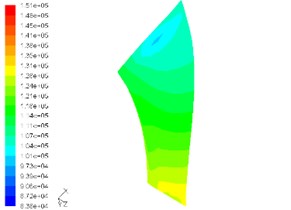
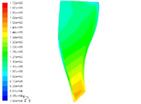
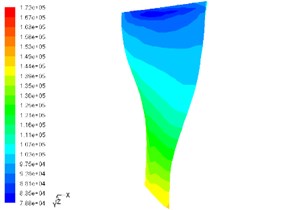
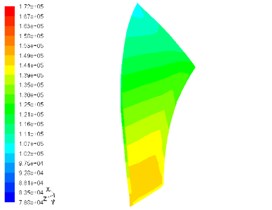
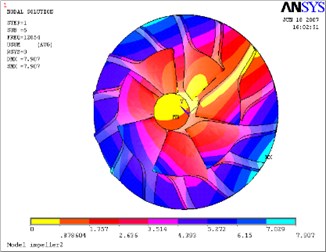
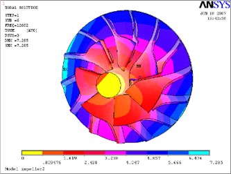
The above Eq. (10) was solved by ANASYS solver with the subspace iteration method. The calculation results of modal parameters are shown in Table 5, with considering the fluid-solid coupled field and the centrifugal stiffening effect. If the modal calculation results of impeller are compared between considering the fluid-solid coupled field and not considering the fluid-solid coupled field, the modal shapes between them are almost the same. But the differences of natural frequencies between them are obvious, and the contrasts are shown in Table 6 and Figs. 12-19.
Table 5Calculation results of modal parameters with considering the fluid-solid coupled field and the centrifugal stiffening effect (at rotating speed of 90,000 rpm)
Mode | Frequencies (in Hz) | Mode characteristics |
1 | 1124.7 | Bending in vertical direction |
2 | 2044.7 | Bending in horizontal direction |
3 | 2335.8 | Bending and torsional coupled |
4 | 10177.0 | Bending in vertical direction |
5 | 11947.0 | Bending in vertical direction |
6 | 12002.0 | Bending in horizontal direction |
7 | 15797.0 | Bending vibration near upper of main blade (partial mode) |
8 | 16350.0 | Bending vibration near upper of main blade (partial mode) |
Table 6Contrasts of natural frequencies between considering the fluid-solid coupled field and not considering the fluid-solid coupled field
Mode | (Not considering coupled, in Hz) | (Considering coupled, in Hz) | Percent of difference between and ((× 100 %) |
1 | 1020.6 | 1124.7 | +10.2 % |
2 | 2611.9 | 2044.7 | –21.7 % |
3 | 3049.5 | 2335.8 | –23.4 % |
4 | 9510.3 | 10177.0 | +7.0 % |
5 | 11733.0 | 11947.0 | +1.8 % |
6 | 12054.0 | 12002.0 | –0.4 % |
7 | 15843.0 | 15797.0 | –2.9 % |
8 | 16457.0 | 16350.0 | –0.6 % |
Fig. 12First mode-impeller
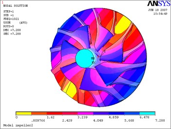
a) Not considering the fluid-solid coupled field
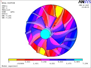
b) Considering the fluid-solid coupled field
Fig. 13Second mode-impeller
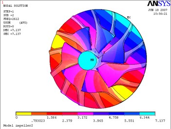
a) Not considering the fluid-solid coupled field
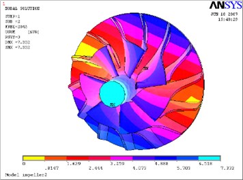
b) Considering the fluid-solid coupled field
Fig. 14Third mode-impeller
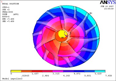
a) Not considering the fluid-solid coupled field
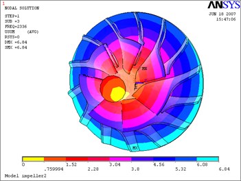
b) Considering the fluid-solid coupled field
Fig. 15Fourth mode-impeller
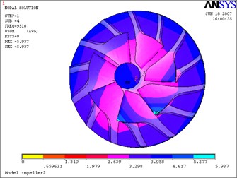
a) Not considering the fluid-solid coupled field
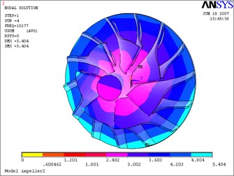
b) Considering the fluid-solid coupled field
Fig. 16Fifth mode-impeller
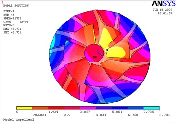
a) Not considering the fluid-solid coupled field
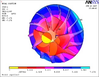
b) Considering the fluid-solid coupled field
Fig. 17Sixth mode-impeller
a) Not considering the fluid-solid coupled field
b) Considering the fluid-solid coupled field
Fig. 18Seventh mode-impeller
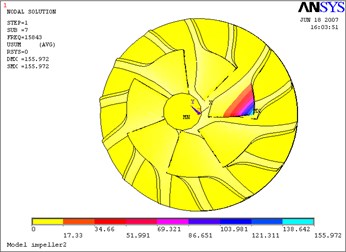
a) Not considering the fluid-solid coupled field
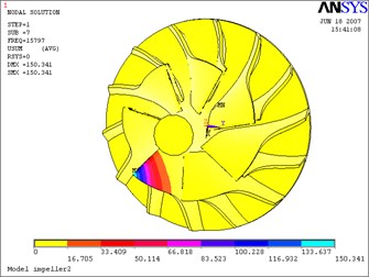
b) Considering the fluid-solid coupled field
Fig. 19Eighth mode-impeller
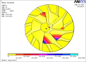
a) Not considering the fluid-solid coupled field
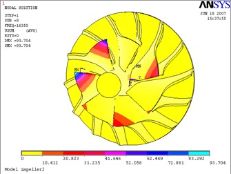
b) Considering the fluid-solid coupled field
4. Conclusions
1) The fluid-solid coupled field has some influences on natural frequencies of impeller and has few influences on its modal shapes. Furthermore, the influences on different natural frequencies of impeller, from the coupled fluid field, are quite different. The natural frequencies of the first mode, fourth mode and fifth mode increase, but the frequencies of the other modes decrease compared with not considering the fluid-solid coupled effects. The coupled fluid field has larger influences on lower modal frequencies than on higher modal frequencies.
2) The differences of the first two modal shapes of impeller between considering the fluid-solid coupled field and not considering the fluid-solid coupled field are small. The first two modal shape coefficients with considering the fluid-solid coupled field are slightly greater. But the modal shape coefficients for the third mode to eighth mode, with considering the fluid-solid coupled field, are slightly smaller than that with not considering the fluid-solid coupled field. It is due to the action of the coupled fluid field which restrains the deformation of higher modes.
3) Since the impeller runs in the range of 60,000 rpm to 180,000 rpm, corresponding to 1,000 Hz to 3,000 Hz, it is essential to consider the effects of the fluid-solid coupled field on the modal frequencies to ensure that the impeller speed is well away from the resonant speeds.
References
-
Motriuk R. W., Harvey D. P. Root cause investigation of the centrifugal compressor pulsation/vibration problems. 4th International Symposium on Fluid-Structure Interactions, Aeroelasticity, Flow-Induced Vibration and Noise, Dallas, TX, USA, 1997, p. 483-489.
-
Kenyon J. A., Griffin J. H., Feiner D. M. Maximum bladed disk forced response from distortion of a structural mode. ASME Journal of Turbomachinery, Vol. 125, Issue 2, 2003, p. 352-363.
-
Shi X., Tang B. Computational investigation of the aerodynamics of automotive turbocharger mixed-flow turbines. Journal of Beijing Institute of Technology (English Edition), Vol. 15, 2006, p. 53-58.
-
Zhang H., Ma C. C. Modeling of centrifugal compressor preliminary design calculations and its performance simulation. Transactions of Beijing Institute of Technology, Vol. 26, Issue 1, 2006, p. 10-13.
-
Zhang H., Ma C. C. Structure computation and analysis of vehicle turbocharger compressor impeller. Chinese Internal Combustion Engine Engineering, Vol. 28, Issue 1, 2007, p. 62-66.
-
Dickmann H. P., Thomas S. W., et al. Unsteady flow in a turbocharger centrifugal compressor: three-dimensional computational fluid dynamics simulation and numerical and experimental analysis of impeller blade vibration. ASME Journal of Turbomachinery, Vol. 128, Issue 7, 2006, p. 455-465.
-
Filsinger D., Szwedowicz J., Schafer O. Approach to unidirectional coupled CFD-FEM analysis of axial turbocharger turbine blades. ASME Journal of Turbomachinery, Vol. 124, Issue 1, 2002, p. 125-131.
-
Filsinger D., Frank C., Schafer O. Practical use of unsteady CFD and FEM forced response calculation in the design of axial turbocharger turbines. ASME Turbo Expo 2005: Power for Land, Sea, and Air, Vol. 4, 2005, p. 601-612.
-
Schmitz M. B., Schafer O., et al. Axial turbine blade vibrations by stator flow-comparison of calculations and experiment. 10th ISUAAAT, Durham, NC, 2003, p. 107-118.
-
Chen Z. H., Liu Y. Q., et al. Vibration characteristic analysis of vehicle turbocharger compressor impeller. Journal of Small Internal Combustion Engine and Motorcycle, Vol. 39, Issue 2, 2010, p. 85-89.
-
Li H. B. Vibration Theory and Its Engineering Application. Beijing Institute of Technology Publishing Press, Beijing, 2006.
-
Ramamurti V., Subramani D. A., Sridhara K. Free vibration analysis of a turbocharger centrifugal compressor impeller. Mechanism and Machine Theory, Vol. 30, Issue 4, 1995, p. 619-628.
-
Han Z. Z., Wang J., Lan X. P. FLUENT Fluid Engineering Simulation Examples and Application. Beijing Institute of Technology Publishing Press, Beijing, 2004.
-
Launder B. E., Spalding D. B. Lectures in Mathematical Models of Turbulence. Academic Press, London, 1972.
-
Li H. B., Zhou J. W., Sun Z. L. Mechanisms and Controls on Noise and Vibration of Automotive Turbocharger. China Machine Press, Beijing, 2012.
-
Zhou L. L. Analysis and Research on Turbocharger Rotor Dynamics. Master’s Degree Thesis, Beijing Institute of Technology, China, 2007.
-
Li H. B., Zhou L. L., et al. Modal analysis of turbocharger impeller considering fluid-solid interaction. Journal of Vibration, Measurement and Diagnosis, Vol. 28, Issue 3, 2008, p. 252-254.
About this article
