Abstract
Numerical simulation approach has recently grown in popularity due to its wide range of applications in the solving of random vehicle-pavement interaction (VPI). This study proposes a framework to simulate the dynamic vehicle load process due to a quarter-truck vehicle model moving along a rough road surface. A procedure used to generate artificial time histories of dynamic vehicle load on road pavement was developed. Example application of the proposed framework is presented and a comparison of calculated and experimental values demonstrates the effectiveness of the framework. To elucidate the relationship between dynamic vehicle load and road roughness, this study normalized the average maximum dynamic vehicle loads on road surfaces of different grades using standard deviation of dynamic vehicle load. Numerical results indicate that the normalized average maximum dynamic vehicle load is not associated with road roughness.
1. Introduction
Vehicle load processes produce various forms of road pavement distress, including fatigue and permanent deformation. Identifying and analyzing the processes involved with vehicle load on road pavements is a random vehicle-pavement interaction (VPI) problem. Numerical simulation approach has recently grown in popularity due to its wide range of applications in the solving of dynamic responses of a pavement structure under moving vehicle loads. Accurately predicting how the pavement responds to vehicle load requires that pavement engineers take into account a wide range of load scenarios.
The load of moving vehicles on a rough road surface has been shown to be stochastic [1, 2], with a strong dependence on the dynamic properties of the vehicle, the speed of the vehicle, and the roughness of the road [3]. Road roughness is widely viewed as a random process and a significant factor in VPI [4]. Hwang and Nowak [5], LaBarre et al. [2], and Marcondes et al. [6] proposed the road spectrum models most commonly used to simulate road roughness. Various vehicle models [7-9] including quarter-truck, half-truck, and full-truck models have been adopted for the analysis of VPI. The selection of vehicle model depends on the specific characteristics of a given problem and influences the precision of analysis results. Todd and Kulakowski [10] indicated that the quarter-truck vehicle model is an appropriate choice for the simulation of dynamic vehicle load caused by VPI.
This study examined how the quality of a road surface influences the maximum dynamic load produced by the vehicle. The findings are meant to elucidate the degree to which road roughness influences dynamic vehicle load and provide a valuable resource for the design and construction of roadways.
2. Vehicular motion
In the following scenario, this study presents a single-axle quarter-truck vehicle with 2-DOFs moving along a rough road from the left to right side at constant speed under the following assumptions: the response of vehicles exhibits linear elasticity; road pavement roughness is a randomly determined stationary Gaussian process with mean of zero; the wheels maintain contact with the surface of the road at all times; and the pavement exhibits negligible deformation, relative to the responses associated with the vibration of the vehicle. In this situation, the only significant factor associated with the vertical vibration of the vehicle is road roughness.
From the perspective of an observer on the vehicle, vertical vibrations in the vehicle as well as the roughness of the road are functions of time . If static vehicle load is not considered, the equation of motion associated with the body of the vehicle can be presented as follows:
where and are respectively the damping and stiffness coefficients of the suspension system; is the sprung mass and is the unsprung mass; is the damping coefficient and is the stiffness coefficients of the tire; is the absolute acceleration, is the absolute velocity, and is the absolute displacement associated with the vertical vibration of the vehicle body; and represents the roughness of the road pavement.
Modal analysis gives the solution of Eq. (1) as follows:
where is the th component of the th mode shape and is the th modal coordinate of the system.
3. Road spectrum
This study proceeded under the assumption that a surface profile of pavement is the manifestation of a random process that can be described using a road spectrum. LaBarre et al. [2] proposed the first road spectrum model:
where , , and are shape coefficients; is circular frequency; is the road roughness coefficient; and is vehicle speed. This study also adopted this model for the simulation of road roughness.
4. Vehicle loads on pavement
Roads with a rough surface can produce vertical vibrations in the body of moving vehicles, thereby transmitting the inertial force associated with the vibration through the suspension system and wheels into the pavement. Dynamic vehicle load can be represented as follows:
In linear systems, if the excitations are a stationary Gaussian random process with zero mean, then the response processes as well as the dynamic vehicle load will also be stationary Gaussian random processes with zero mean. Thus, we can substitute Eq. (2) into (4) to obtain:
Estimating dynamic vehicle load makes it possible to calculate the total vehicle load using the following equation:
5. Dynamic vehicle load spectrum
In accordance with the theory of random vibration, Lin [11] proposed a closed-form solution for the dynamic vehicle load spectrum :
where is the th modal damping ratio of the system and is the undamped natural frequency of the th modal.
6. Generating a time history of dynamic vehicle load
The closed-form solution for in Eq. (7) can be utilized to simulate the time history of dynamic vehicle load for pavement response analysis. The methods used in the analysis of pavement structures under a moving vehicle load can be classified into two categories: theoretical and numerical. In theoretical study, the dynamic load process of vehicles may be described by the . This approach makes it possible to obtain an exact solution; however, some of the assumptions made during analysis can limit its applicability. In numerical simulation, the dynamic processes associated with the load of vehicles can be described in historical terms generated artificially from , using Monte Carlo simulation.
Modelling dynamic load processes as stationary, random, Gaussian processes with a zero mean makes it possible for them to be generated using an inverse Fourier transform as follows:
where is a random phase angle uniformly distributed from 0 to 2; is circular frequency; the frequency increment ; and is the total number of frequency increments within the frequency interval (, ) in which is defined. and are the maximum and minimum frequencies, respectively. A superposition of harmonics with random phases is represented in Eq. (10), which makes it possible to generate artificial sample functions from a particular ensemble spectral density function of a stationary random process.
7. Numerical examples
Numerical examples were generated by considering a single-axle, quarter-truck vehicle model with 2-DOFs moving at a speed of 90 km/h (25 m/s). This study selected the following parameters for the vehicle model: 5000 kg, 500 kg, 500 kN/m, 2000 kN/m, and 11.07 kN∙s/m. The corresponding vibration frequencies of the vehicle model were 8.9 rad/s and 70.9 rad/s. Road roughness was treated as the primary factor in VPI. This study used the LaBarre road spectrum model for the simulation of pavement roughness, using the parameter values proposed by Dodds and Robson [1] for road surfaces with a variety of grades on minor roads, principal roads, and motorways. The associated dynamic vehicle load spectra were estimated from Eq. (7).
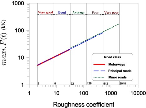
Simulation methods are commonly used for the estimation of the extremes associated with random processes. This study generated a time history of dynamic vehicle load using the procedures outlined in previous section. As shown in Figs. 1(a) to 1(d), four typical load histories were generated using the selected parameters for which we sought to obtain the maximum values. Statistical analysis on the maximum dynamic vehicle loads was used to obtain the average maximum dynamic vehicle load based on 30 artificially generated histories of dynamic vehicle load. The results revealed that a four-fold increase in the road roughness coefficient resulted in a two-fold increase in the average maximum dynamic vehicle load, as shown in Fig. 2.
Fig. 1Typical simulated time history of dynamic vehicle load moving over principal roads of four different grades at a vehicle speed of 90 km/h
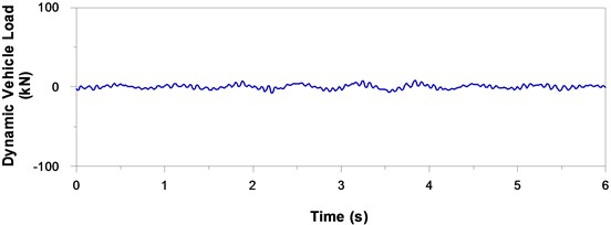
a) Very good
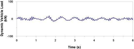
b) Good

c) Average
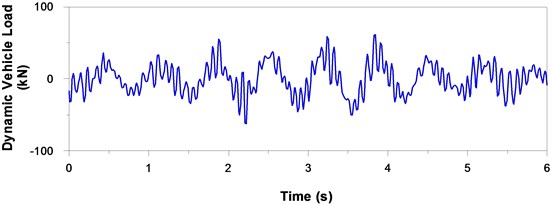
d) Poor
Fig. 2Relationship between maximum dynamic vehicle load and the grade of surfaces on roads of various classes
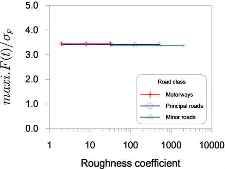
The accuracy of the results was evaluated by comparing them with experimental data. Fig. 3 illustrates the relationship between the normalized average maximum dynamic vehicle load, , and road roughness coefficient for roads of various classes. The values of ranged between 3.36 and 3.44 for roads of various classes. Hahn [12] reported that peak dynamic loads generally exceed the standard deviation of the dynamic load by a factor of approximately 3. These results also reveal that is unconnected to the roughness of the road.
The magnitude of the dynamic vehicle loads is principally a function of pavement-surface roughness at a specified speed. This study used the dynamic load coefficient (DLC) as a parameter for characterizing the magnitude of dynamic vehicle load, defined as follows:
Fig. 3Relationship between normalized maximum dynamic vehicle load and road roughness coefficient for roads of various classes
In Table 1, this study presents the results for the DLC of road surfaces of various grades from poor to good, ranging 0.08 to 0.38. Under normal operating conditions, we could expect DLCs of 0.1 to 0.3 for VPI [13]. In particularly poor conditions, Sweatman [14] measured values as high as 0.4.
Table 1Dynamic load coefficient for different grades of road surface on motorways, principal roads, and minor roads
Road class | Grade of road surface | Roughness coefficient | Dynamic load coefficient (DLC) |
Motorways | Good | 20 | 0.08 |
Principal roads | Good | 20 | 0.09 |
Average | 80 | 0.18 | |
Poor | 320 | 0.36 | |
Minor roads | Average | 80 | 0.19 |
Poor | 320 | 0.38 | |
measured in units of 10-6 (m3/cycle). | |||
8. Conclusions
This study is concerned with simulation of dynamic vehicle load on road pavement resulting from the interaction between a quarter-truck vehicle and road surface roughness. A comparison of calculated and experimental values related to the statistical characteristics of dynamic vehicle load demonstrates the effectiveness of the proposed framework. It is concluded that a four-fold increase in the road roughness coefficient results in a two-fold increase in the maximum dynamic vehicle load . This study also determined that the normalized average maximum dynamic vehicle load is not associated with road roughness.
References
-
Dodds C. J., Robson J. D. The description of road surface roughness. Journal of Sound and Vibration, Vol. 31, 1973, p. 175-183.
-
LaBarre R. P., Forbes R. T., Andrew S. The measurement and analysis of road surface roughness. Motor Industry Research Association, Report No. 1970/5, Nuneaton, England, 1970.
-
Ullidtz P. Pavement Analysis. Elsevier, New York, 1987.
-
Sawant V. Dynamic analysis of rigid pavement with vehicle-pavement interaction. International Journal of Pavement Engineering, Vol. 10, 2009, p. 63-72.
-
Hwang E. S., Nowak A. S. Simulation of dynamic load for bridges. Journal of Structural Engineering, Vol. 117, 1991, p. 1413-1434.
-
Marcondes J., Burgess G. J., Harichandran R., Snyder M. B. Spectral analysis of highway pavement roughness. Journal of Transportation Engineering, Vol. 117, 1991, p. 540-549.
-
Hrovat D. Influence of unsprung weight on vehicle ride quality. Journal of Sound and Vibration, Vol. 124, 1988, p. 497-516.
-
Zhong Y., Liu J. Theoretical analysis of random dynamic load between road and vehicle. Engineering Mechanics, Vol. 10, 1993, p. 26-31.
-
Nielsen J. C. O., Igeland A. Vertical dynamic interaction between train and track: influence of wheel and track imperfections. Journal of Sound and Vibration, Vol. 187, 1995, p. 825-839.
-
Todd K. B., Kulakowski B. T. Simple computer models for predicting ride quality and pavement loading for heavy trucks. Transportation Research Record 1215, TRB, National Research Council, Washington, US, 1991, p. 137-150.
-
Lin J. H. Variations in dynamic vehicle load on road pavement. International Journal of Pavement Engineering, Vol. 15, 2014, p. 558-563.
-
Hahn W. D. Effects of Commercial Vehicle Design on Road Stress – Quantifying the Dynamic Wheel Loads for Stage 3: Single Axles, Stage 4: Twin Axles, Stage 5: Triple Axles, As a Function of the Springing and Shock Absorption System of the Vehicle. Report No. 453, Institut fur Kraftfahrwesen, Universitat Hannover, Germany, 1987.
-
Sweatman P. F. Effect of Heavy Vehicle Suspensions on Dynamic Road Loading. Research Report ARR, No. 116, Australian Road Research Board, Vermont South, Victoria, Australia, 1980.
-
Sweatman P. F. A Study of Dynamic Wheel Forces in Axle Group Suspensions of Heavy Vehicles. Special Report No. 27, Australian Road Research Board, Vermont South, Victoria, Australia, 1983.
About this article
