Abstract
A numerical implementation of two-way collinear interaction of nonlinear ultrasonic longitudinal waves in an elastic medium with quadratic nonlinearity is conducted in this work. A semi-discrete central scheme is used here to solve the numerical problem. The pulse-inversion technique is applied to accentuate the generated resonant waves and remove the fundamental components. The produced resonant waves can be clearly observed in the frequency domain. Variation trends of the resonant waves together with second harmonics along the propagation path are analyzed and results show that apart from the obvious growing of the transverse component with difference frequency, the longitudinal component and the resonant wave of sum frequency have notable responses as well. The spatial distribution of resonant waves will provide necessary information for the related experiments.
1. Introduction
Nonlinear ultrasonic nondestructive evaluation (NDE) techniques have attracted plenty of attention due to their sensitivity to characterize early damage in recent years, among which the wave mixing technique is relatively new. Nonlinear interaction between intersecting waves caused by material nonlinearities was firstly investigated in the 1960s [1-3], and theoretically studied more recently by Chen et al. [4], Kuvshinov et al. [5] and Korneev and Demčenko [6]. Liu et al. [7, 8] and Tang et al. [9] develop a collinear wave mixing method to measure the acoustic nonlinearity parameter and detect localized plastic deformation. Croxford et al. [10] and Demčenko et al. [11, 12] carried out experimental researches of the technique to detect plasticity and fatigue of metal alloys and physical aging of polymers, respectively.
The wave mixing technique is based on the fact that under certain circumstances, two elastic propagating waves in a nonlinear solid may interact and produce a third propagating wave of sum or difference frequency. This third propagating wave is called the resonant wave. The technique has been demonstrated to possess some unique advantages over other nonlinear NDE methods. Firstly, effective selectivity of frequency, mode, direction and space can be realized. Secondly, system nonlinearity can be both independently measured and enormously eliminated. Thirdly, both single and double edge access are suitable for a practical application. Compared with non-collinear wave mixing, collinear wave mixing enables convenient scanning over a region of interest and saves angle conversion of transducers.
Although the technique of wave mixing technique has been focused on by many researchers, there have not been specific studies on direct comparison of resonant waves and second harmonic waves when coexisting. Meanwhile, the wave type of the resonant wave is also of interest to be reexamined, and the variation trend of it along the whole propagating path waits to be revealed. With these in question, a numerical simulation concentrated on the wave mixing process is worth studying for a better understanding of the phenomenon.
Based on an appropriate high-resolution central scheme, a numerical study of anti-linear mixing of nonlinear waves in an elastic medium is implemented. The obtained numerical results are analyzed and evaluated in time and frequency domain, followed by a comparative research of variation trends of the produced resonant waves.
2. Modeling of wave propagation in an elastic solid with quadratic nonlinearity
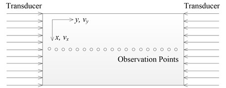
Quadratic nonlinearity is widely employed to characterize hyper-elasticity of a material, corresponding to lattice anharmonicity of elastic solids. Severe dislocation induced deformation is not considered here. Consider a pair of two-way collinear plane waves propagating in opposite directions in an elastic medium with quadratic nonlinearity. Without loss of generality, assume the waves are propagating along the direction in a Cartesian coordinate system (, , ). Two coupled hyperbolic partial differential equations are introduced to describe wave propagation, and two time-dependent line loads are applied on the boundary 0, and (, ). Symmetry of the problem leads to a two-dimensional motion governed by a second-order hyperbolic system of partial differential equations as follows:
where , , represents stress components, and represent displacement components in and directions, respectively, and represents the density of the material. The boundary conditions for the problem are given by:
where is the delta function representing the line load, , , , denote Cartesian coordinate components of two excitation sources respectively, and denote the temporal input signal functions of two transducers respectively both of which can be given by:
is the amplitude of . Displacements and velocities of particles in the half space are all set to be zero at time zero.
Consideration of only small strain deformations results in the neglect of terms of the geometrical nonlinearity, and the corresponding constitutive equations can be given by [13, 14]:
where , are second-order elastic constants, and , are third-order elastic constants.
3. Numerical solution
The considered nonlinear problem can be conveniently reformulated into a hyperbolic system of conservation laws defined on a two-dimensional domain as follows:
where is the state vector which is represented as:
And structures of two flux vectors and are:
Unlike a linear stress-strain relationship that the Jacobian matrices and have real eigenvalues, for a nonlinear case, the matrices may have complex eigenvalues. The hyperbolicity of Eq. (5) can be guaranteed by adjusting the input amplitude on the boundary. Eq. (5) can be solved by either an explicit second-order Runge-Kutta method or the modified Euler method. In this work, a high-resolution second-order central scheme proposed by Kurganov and Tadmor [15] is considered as a numerical solution algorithm applied in the propagation problem, and the numerical solution algorithm is implemented using the library CENTPACK [16] with some improvements. A ghost-cell method [17] which has been integrated into CENTPACK is introduced here to implement the boundary conditions. From a comparison by Küchler et al. [13], it can be seen that the numerical solution and the exact analytical one are in good agreement. And it is also shown that the solution procedure used here offers a high-resolution solution for wave propagation in both linear and nonlinear elastic half-spaces [14]. The material parameters used here correspond to Aluminum D54S [18] and are given in Table 1.
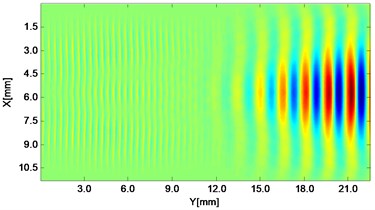
Fig. 1Two wave mixing in a nonlinear solid (11.25 mm×22.5 mm)
4. Simulation results and discussions
There are mainly three types of intersection cases of wave mixing, which are two transverse waves, two longitudinal waves and one transverse and one longitudinal wave, respectively. And in this work, the two-way collinear mixing of longitudinal waves is mainly involved. The pulse-inversion technique is applied to reduce the dominance of the fundamental contribution [19]. Not only are the even order harmonics extracted by combining two reciprocal phased input signals, but also the resonant waves of sum and difference frequencies are found to be accentuated in the meantime. In order to observe the resonant wave independently, the frequencies of two primary waves have to be appropriately chosen, which should keep away from frequencies of fundamental components of primary waves as well as those of generated harmonics. Base on the consideration mentioned, one pair of 2 MHz and 7.6 MHz is selected as driving frequencies.
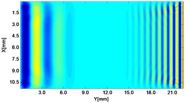
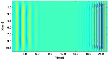
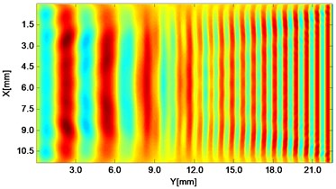
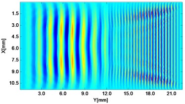
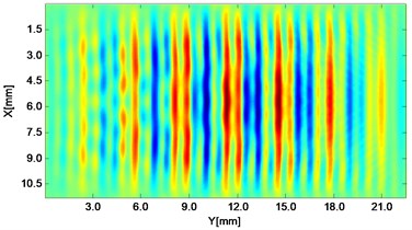
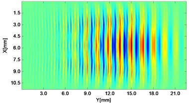
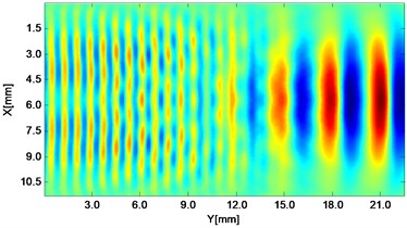
Fig. 2Propagating wave fronts of vy in a nonlinear medium at different times, corresponding to original and combined responses, respectively
a)1.5 μs
b)1.5 μs
c)3.0 μs
d)3.0 μs
e)4.5 μs
f)4.5 μs
g)6.0 μs
h)6.0 μs
4.1. Wave fronts in the whole field
Wave fronts of particle velocity in the direction are plotted at four different times. At the very beginning the two stress waves just leave away from the boundaries Fig. 2(a), and then they meet each other in the middle of the structure and the interaction process starts Fig. 2(c). At a later time, as two primary waves propagate further, the wave fronts change their width, interval and peak-valley array pattern due to the wave interaction Fig. 2(e). Finally, the two incident waves separate apart leaving the whole wave field appeared to be more complicated Fig. 2(g). The combined responses are also plotted in Fig. 2 corresponding to these four times, respectively. Second harmonics can be observed from their twice denser stripes compared with those of primary waves. Besides, as seen between two groups, the harmonic waves propagate roughly synchronously with the fundamental waves. Similarly, wave fronts of particle velocity in the direction at the four times mentioned can also be plotted. Unlike the axial symmetry of responses in the direction, those in the direction appear to be axial anti-symmetric about the central horizontal line, i.e. each pair of symmetrical points in the upper and lower part basically have opposite values. Additionally, shapes of wave fronts are not straight but curved.
Fig. 3Numerical solution of particle velocities in a nonlinear medium at different locations along the direction of the resonant wave propagation
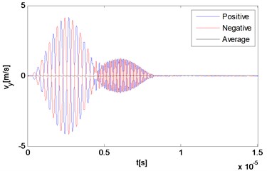
a) 0.45 mm
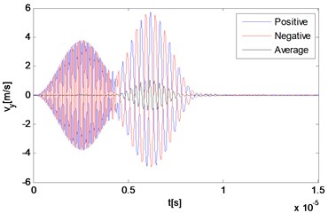
b) 22.05 mm
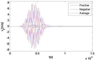
c) 11.25 mm
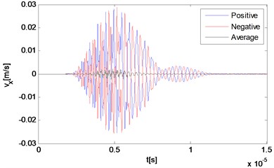
d) 11.25 mm
4.2. Responses in time domain
The reciprocal phased outputs and their average values are plotted together in Fig. 3 with three representative locations. As Fig. 3(a) and 3(b) show, because of the time difference, responses of locations far away from the interaction zone manifest separate waveforms corresponding to the primary waves respectively, although the second part of each one has already been effected by the wave interaction phenomenon. The two reciprocal phased outputs have roughly opposite values at each time, and the average part also can be clearly observed within the second waveform in Fig. 3(b). The third point locates rightly in the center of the intersection zone where two primary waves mix thoroughly. Because two input signals are set to be of the same length, waves propagating across this point keep containing more than one frequency component all the time. It can be seen from Fig. 3(c) and 3(d) that due to the wave interaction, the whole output waveform is completely distorted compared with those of input primary waves.
4.3. Responses in frequency domain
As the technique of wave mixing mainly utilizes information of the frequency components, fast Fourier transform (FFT) of velocity output is conducted to obtain the responses in the frequency domain. Firstly, the middle point is selected again and its particle velocity in and directions are plotted in Fig. 4(a) and 4(b), respectively. It can be seen that at this point, the two main components are related with two second harmonics of primary waves, which are 4 MHz and 15.2 MHz respectively, and far more noticeable than those of resonant waves, which are 5.6 MHz and 9.6 MHz respectively. Besides, the difference resonant component 5.6 MHz appears more obvious in the direction than direction. In order to make sure whether the resonant wave grows as propagating to the left side of the structure, another two observation points are selected for a comparison. When the wave propagates half way from middle to the left end, its amplitude has increased both in absolute value and relative value to those of the second harmonic waves (Fig. 4(c)). Finally, before it reaches the left end, its amplitude has already dominated the whole frequency domain, when other frequency components have become much more unremarkable as shown in Fig. 4(d).
Fig. 4FFT of particle velocities in a nonlinear medium at different locations along the direction of the resonant wave propagation
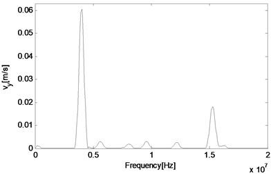
a) 11.25 mm
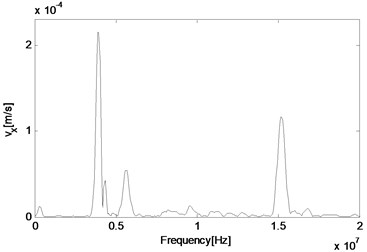
b) 11.25 mm
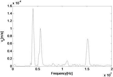
c)5.85 mm
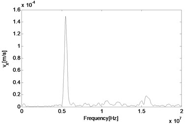
d) 0.45 mm
4.3.1. Variation trend of resonant waves
After observing the generated resonant wave with both sum and difference frequencies, it is able to obtain the variation trend of the resonant wave along the propagating path. According to the interaction condition of two-way collinear cases, two longitudinal waves can generate a SV wave propagating along the path of the primary wave with the higher frequency. It is of much interest to see how the generated resonant wave behaves at each point when propagating, and also whether other types of waves such as a longitudinal wave can be generated simultaneously.
Compared with cases of non-collinear interaction when paths of observation points need to be carefully selected, here waves propagate mainly along one specific line. 37 equidistant observation points are chosen on the central line of the propagation path, and the 19th point locates at the interaction zone where two primary waves meet with each other. The distance between adjacent points is 0.6 mm.
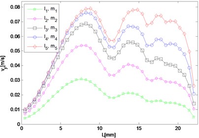
Fig. 5Spatial distribution of resonant and harmonic waves
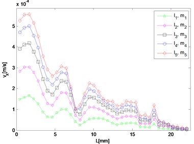
a) 5.6 MHz
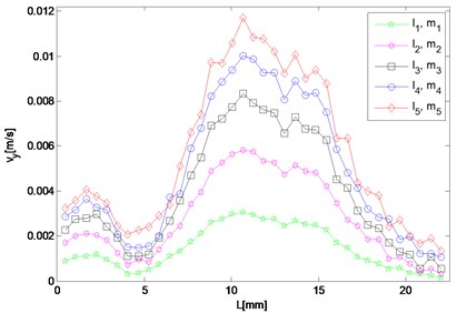
b) 5.6 MHz
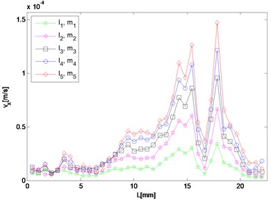
c) 9.6 MHz
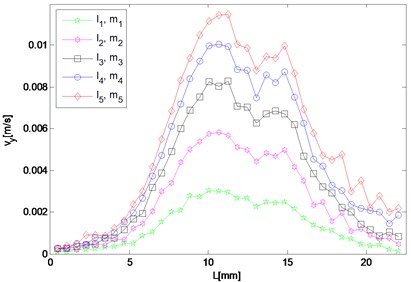
d) 9.6 MHz
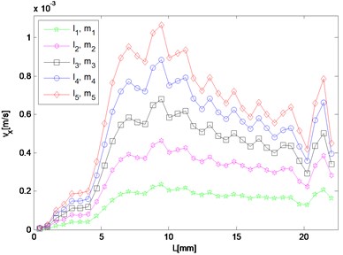
e) 4 MHz
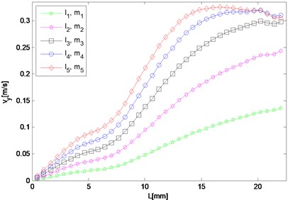
f) 4 MHz
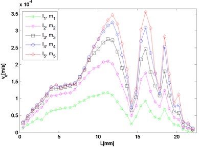
g) 15.2 MHz
h) 15.2 MHz
For frequency component of resonant waves and second harmonic waves, although the response in either or direction needs to be investigated respectively, results in both directions are given here as potential supplement. In the case, the difference and sum resonant frequencies are 5.6 MHz and 9.6 MHz respectively, and 4.0 MHz and 15.2 MHz for the second harmonics respectively. Five different sets of nonlinearity parameters are applied to provide a comparison, of which one set describes the intact material, and the other four sets characterize ones with fatigue damage at different stages.
It can be seen in Fig. 5(a) that the amplitude of 5.6 MHz component in the direction reaches maximum near the left end and meantime diminishes approaching the right end, which means that after a transverse resonant wave is actually generated, it propagates towards the left way along the direction the same as that of the primary wave of the larger driving frequency. For the 9.6 MHz component, its amplitude increases only when the wave propagates to the right and two peaks appear round 15 mm and 18 mm respectively (Fig. 5(c)). By contrast, it decays as coming close to the left end. Fig. 5(b) and 5(d) show amplitudes of the resonant waves in the direction, which manifest a similar variation trend. Both of them reach maximum at about 11 mm in the middle of the structure, and decrease when propagating either to the left or right end. The peak values of difference and sum frequency cases are nearly the same, and roughly 20 and 70 times of those in the direction, respectively.
Responses of second harmonic waves are not of main concern here, but as frequency components they are together with resonant waves constituting the whole frequency spectrum, and therefore amplitudes of harmonic components in and directions are also displayed in Fig. 5(e) to 5(h) so that the resonant responses mentioned above can be analyzed by comparing with them. It is noted that in the direction, both amplitudes of harmonic waves gradually decrease from the middle interaction zone to the left side where that of the difference frequency resonant wave dominates the whole frequency domain. While in the direction, the harmonic components appear more prominent than the resonant ones at most observation points.
As for responses corresponding to different levels of nonlinearity parameter input, it can be found in Fig. 5 that amplitudes of almost all the observation points increase monotonically with third-order elastic constants and . The larger and are given to be, at the slower rate the nonlinear response grows, which means the resonant response varies more remarkably when the nonlinearity starts to grow from the original state of the material.
5. Conclusions
A numerical calculation of two-way collinear mixing of longitudinal waves in an elastic medium is investigated in this work. The pulse-inversion technique applied here is proved effective to filter out the fundamental components and accentuate the higher order harmonics as well as the generated resonant waves. Here two second harmonics and two resonant waves of sum and difference frequencies are analyzed and compared with each other in the same frequency domain. Generation location and variation trend of the resonant waves are examined along the whole propagating path, and it is found that not only a vertical transverse wave but also a longitudinal wave can be produced under appropriate circumstances, of which the former is observed to be more significant in the propagating direction of the primary wave with the higher frequency.
As for applicability and benefit of the presented technique for real life NDE applications, there are mainly three aspects as follows. Firstly, it provides variation trends of resonant waves with separate cases of different nonlinearity parameter inputs, which contributes to material characterization by establishing a nonlinear relationship between states of material and elastic constants; Secondly, based on results of intensity distribution of resonant waves, the triggering time can be adjusted in order to obtain a strong response of resonant component on the boundary; Thirdly, the technique of pulse-inversion is demonstrated to be of potential value for being applied in the related experiments.
This numerical study has demonstrated that a frequency spectrum of second harmonics and resonant waves of a pair of primary waves can be independently extracted and observed, showing a clear comparison and contrast between them. It will contribute to optimization of related experimental configurations, especially in measuring the nonlinearity parameters and detecting fatigue damage at early stages.
References
-
Jones G. L., Kobett D. R. Interaction of elastic waves in an isotropic solid. The Journal of the Acoustical Society of America, Vol. 35, 1963, p. 5-10.
-
Rollins F. R. Interaction of ultrasonic waves in solid media. Applied Physics Letters, Vol. 2, 1963, p. 147-148.
-
Taylor L. H., Rollins F. R. Ultrasonic study of three-phonon interactions. 1. Theory. Physical Review Letters, Vol. 136, 1964, p. 591-596.
-
Chen Z., Tang G., Zhao Y., et al. Mixing of collinear plane wave pulses in elastic solids with quadratic nonlinearity. The Journal of the Acoustical Society of America, Vol. 136, Issue 5, 2014, p. 2389-2404.
-
Kuvshinov B. N., Smit T. J. H., Campman X. H. Non-linear interaction of elastic waves in rocks. Geophysical Journal International, Vol. 194, Issue 3, 2013, p. 1920-1940.
-
Korneev V. A., Demčenko A. Possible second-order nonlinear interactions of plane waves in an elastic solid. The Journal of the Acoustical Society of America, Vol. 135, Issue 2, 2014, p. 591-598.
-
Liu M., Tang G., Jacobs L. J., Qu J. Measuring acoustic nonlinearity by collinear mixing waves. Review of Progress in Quantitative Nondestructive Evaluation, Vol. 1335, 2011, p. 322-329.
-
Liu M., Tang G., Jacobs L. J., Qu J. Measuring acoustic nonlinearity parameter using collinear wave mixing. Journal of Applied Physics, Vol. 112, 2012, p. 024908.
-
Tang G., Liu M., Jacobs L. J., Qu J. Detecting localized plastic strain by a scanning collinear wave mixing method. Journal of Nondestructive Evaluation, Vol. 33, 2014, p. 196-204.
-
Croxford Anthony J., Wilcox Paul D., Drinkwater Bruce W., Nagy Peter B. The use of non-collinear mixing for nonlinear ultrasonic detection of plasticity and fatigue. The Journal of the Acoustical Society of America, Vol. 126, Issue 5, 2009, p. 117-123.
-
Demcenko A., Akkerman R., Nagy P. B., Loendersloot R. Non-collinear wave mixing for non-linear ultrasonic detection of physical ageing in PVC. NDT&E International, Vol. 49, 2012, p. 34-39.
-
Demcenko A., Koissin V., Korneev V. A. Noncollinear wave mixing for measurement of dynamic processes in polymers: physical ageing in thermoplastics and epoxy cure. Ultrasonics, Vol. 54, Issue 2, 684, p. 693-2014.
-
Küchler Sebastian, Meurer Thomas, Jacobs Laurence J., Qu Jianmin Two-dimensional wave propagation in an elastic half-space with quadratic nonlinearity: a numerical study. The Journal of the Acoustical Society of America,Vol. 125, Issue 3, 1293, p. 1301-2009.
-
Küchler Sebastian Wave Propagation in an Elastic Half-Space with Quadratic Nonlinearity. M.S. Thesis, Georgia Institute of Technology, Atlanta, GA, 2007.
-
Kurganov A., Tadmor E. New high-resolution central schemes for nonlinear conservation laws and convection-diffusion equations. Journal of Computational Physics, Vol. 160, 2000, p. 241-282.
-
Balbás J., Tadmor E. CENTPACK, available at http://www.cscamm.umd.edu/centpack/software
-
Leveque R. J. Finite Volume Methods for Hyperbolic Problems, Cambridge Texts in Applied Mathematics. Cambridge University Press, Cambridge, 2002.
-
Smith R. T., Stern R., Stephens R. W. B. Third-Order elastic moduli of polycrystalline metals from ultrasonic velocity measurements. The Journal of the Acoustical Society of America, Vol. 40, Issue 5, 1002, p. 1008-1966.
-
Kim Jin-Yeon, Jacobs Laurence J., Qu Jianmin Experimental characterization of fatigue damage in a nickel-base superalloy using nonlinear ultrasonic waves. The Journal of the Acoustical Society of America, Vol. 120, Issue 3, 1266, p. 1273-2006.
About this article
The authors would like to gratefully acknowledge the supports received from the National Natural Science Foundation of China (NSFC No. 11372179) and Program for New Century Excellent Talents in University (NCET-13-0363).
