Abstract
The parameters of elliptical tank can greatly affect the roll stability of the elliptical tank with different filled levels, the exact equations for the mass centre of the tank were developed. The solutions of the transient mass centre of sloshing liquid in a tank with modified elliptical cross sections were obtained by a new vehicle rollover model. To achieve Euler transform 6-degree of freedom (DOF) motion equation of tank, Liquid Sloshing model of partially-filled tank was built by Nonlinear External Excitation. In addition, MATLAB ODE was used to investigate the numerical simulation. According to the different filled level of the tank by simulating, force and moment about , and -axis of the coordinates of the mass centre were obtained. It is shown that the nonlinear mathematical models of liquid sloshing and vehicle motion equation can accurately describe the tank truck dynamic response in turing. The finding of this study may provide a theoretical basis to improve the roll stability of the tank.
1. Introduction
Truck crashes are particular importance because the size and weight of these vehicles results in a greater likelihood of fatalities when they are involved in a crash compared to passenger cars. Truck accidents in the state of New Jersey represent about 8 percent of all accidents. In 1998, 1999, and 2000, there were 20,025, 21,561, and 28,328 accidents respectively, involving trucks in the State. These accidents represent all fatal, injury and property damage accidents for all types of trucks, with the majority of these accidents property damage accidents [1]. And a US study has reported that the average annual number of cargo tank rollovers is about 1265, which takes up 36.2 % in the total number of heavy vehicle highway accidents [2]. Although there are many reasons that lead to tank vehicle rollover accidents, such as driver’s fatigue, overtaking, bad road and weather conditions, and so forth, liquid sloshing in the tank are the main factors [3, 4].
Liquid sloshing inside partially filled containers has been investigated extensively in the aerospace field in the 1950’s and 1960’s. The purpose was to study the effect of partially filled fuel tank of different shapes on the stability of rockets and airplanes. Several mathematical models as well as equivalent mechanical models have been developed to simulate liquid sloshing effects in partially filled containers. The use of simple and compound pendulums has been proved successful in simulating liquid-sloshing effects in partially filled containers of various shapes, especially spherical and cylindrical.
The roll stability of a partially filled tank is influenced by both the centre of gravity (C.G.) height and the magnitude of lateral load transfer. Differential cross sections have been analysed to optimize the roll stability of the tank. The circular cross section has a high centre of liquid location, but considerably less lateral load transfer with low filled volumes under a steady turning lateral acceleration field. On the other hand, modified elliptical tank compared to circular tank yield lower C.G. Height and relatively larger lateral load transfer with low filled volumes. Therefore, the modified elliptical tank represents higher roll stability limits than a circular tank [5].
Sloshing forces depend on the freedom that the liquid has to move into the tank, and on the amount of liquid participating in the motion. While such freedom of movement of the liquid is characterized by the free surface dimensions of the liquid, the amount of moving liquid depends on the filled level of the tank. Because the tank used for carrying liquids have in general a non-rectangular cross section, e.g. elliptic, modified elliptic and circular, the filled level will define the amount of moving liquid and the size of the free surface of the liquid [6].
Many studies have been carried out on liquid flow and sloshing characteristics that happened in the tank. The main methods are the quasi-static (QS) method and the experimental method. The cargo’s static moment at a specified point on a tank vehicle can be approximated by calculating the transient C.G. of the liquid in the tank. Then, the liquid sloshing effect on tank walls can be analysed. It is convenient and simple to obtain liquid sloshing force using the QS method. However, the analysis results have poor accuracy [7-9]. The experimental method, by building a test platform or using test tank vehicles, liquid sloshing phenomenon can be observed and relevant parameters can be monitored by reproducing liquid sloshing [10-11].
In a word, QS method is simple and intuitive and can be used for approximate calculation, but the accuracy is not high. The equivalent mechanical model in the impact of liquid in the tank was more accurate than the QS method. When the liquid impact is large amplitude, the study should be nonlinear coupled with liquid shock. Thus, the aim of this study is to 1) establish liquid free surface equation of motion, 2) set up model of liquid sloshing force and moment caused by nonlinear excitation, two models coupling to take simulate result, could be real reaction tank liquid sloshing situation.
2. The theoretical model
2.1. The free-surface equilibrium formulation of the liquid within a tank
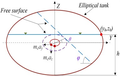
The elliptical tanks overturning moment for liquid goods is caused by lateral and vertical displacement, those are the potential influencing factors of the vehicle roll. Steady state shifting of the liquid cargo C.G. has been modelled by different approaches, including geometrical modelling and experimental methods [11]. We would like to solve the equation of the elliptical cross section mass centre of the tank. Elliptical tank under a steady lateral acceleration field as shown in Fig. 1. The Angle is the between the horizontal direction and the free surface, changed the range is 0 to 90°, that is above 30° belongs to large amplitude.
The third and fifth order vibration modes are antisymmetric wave. Under this three order mode, liquid vibration can lead to C.G. of the lateral displacement. The fourth and sixth order vibration modes are symmetric wave. Under these three modes, liquid vibration will not be able to make C.G. lateral displacement. In addition, the vast majority of liquid C.G. happens larger displacement under the sloshing of first order modal. But the third order and fifth order modal, the size of the maximal displacement and displacement of the liquid C.G. number is greatly reduced. Therefore, under the sloshing of first order modal, liquid C.G. displacement is the largest. In a word, the first-order sloshing model is the lateral sloshing of the liquid in the tank is the most important modal. Furthermore, the sloshing effects can be described by liquid C.G. displacement. The first order model of the liquid free surface can be described by the inclined plane to approximate.
The and position of the liquid cargo C.G., as shown in Fig. 1.
is defined as:
The slope of the liquid along the corresponding ellipse, is:
The C.G. position of the liquid depends on the free surface factors such as slope and cross section shape of tank, ignore the mass center of liquid along the longitudinal axis of the tank on the small changes that the cross section of the C.G. position of the same uniform distribution of liquid in the tank, there is no density difference.
The liquid C.G. position is given by:
1) , the filled level is 0 to 50 %, and , the slope of the C.G. ellipse:
2) , the filled level is 50 % to 100 %, , the slope of the C.G. ellipse:
The liquid C.G. position is given by:
Fig. 1Elliptical tank under a steady lateral acceleration field
Assumptions made include neglecting of sloshing damping. However, the most important simplification in the model is the uncoupled response of the liquid cargo with the truck. In that respect, it could be expected that the coupled sloshing frequency could be lower than the calculated, due to truck suspensions deformation. Hence, liquid sloshing frequency and is much less than the natural tanker vibration frequency. The resonance phenomenon can be ignored.
Due to , the filled level f is in the 50 % to 100 %, and the roll angle 5° remains the same, the elliptic diameters is 2. 2 m and 1. 6 m, the circular diameter is 0.94 m. The coordinates of the axis and axis change with the lateral acceleration () are shown in Fig. 2. Liquid C.G. height and lateral displacement in different filled level change with the lateral acceleration () and the liquid in the tank with ay all show a trend of rising, but higher filled level liquid mass centre height range is smaller, smoother. Compared with the cross section area of the circular tank, the elliptical cross section of tank centre of mass is lower. As Fig. 2 shown, circular cross section and the elliptical cross section in the equal area, the circular cross section of the axis coordinate values have been maintained a higher height of mass centre. As the condition of an equivalent filled level, an elliptical cross section of tank car has better roll stability than the circular.
Fig. 2The values of ay/z, y/z
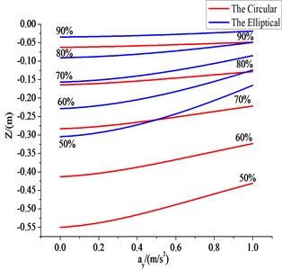
a) The values of
b) The values of
2.2. The liquid sloshing model of partially-filled tank
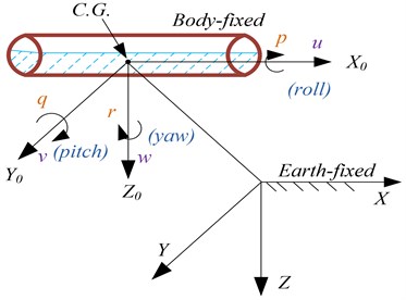
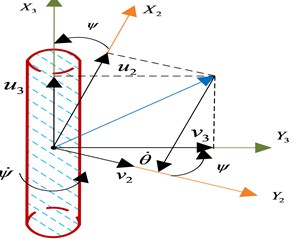
When analysing the motion of the tank in 6-DOF, it is convenient to define two coordinate frames as indicated in Fig. 1. The moving coordinate frame is conveniently fixed to the vehicle and is called the body-fixed reference frame. The origin of the body-fixed frame is usually chosen to coincide with the C.G. When C.G. is in the principal plane of symmetry or at any other convenient point if this is not the case. For tank, the body axes , and coincide with the principal axes of inertia, and are usually defined as:
– longitudinal axis (directed from aft to fore), – transverse axis (directed to board), –normal axis (directed from top to bottom).
Table 1Notation used for the tank
DOF | Forces and moments | Linear and angular velocity | Position and Euler angles | |
1 | -direction (surge) | |||
2 | -direction (sway) | |||
3 | -direction(heave) | |||
4 | Rotation about -axis (roll) | |||
5 | Rotation about -axis (pitch) | |||
6 | Rotation about -axis (yaw) |
The motion of the body-fixed frame is described relative to an inertial reference frame. For tank, it is usually assumed that the accelerations of a point on the surface of the Earth can be neglected. Indeed, this is a good approximation since the motion of the Earth hardly affects slow speed tank. As a result of this, an earth-fixed reference frame can be considered to be inertial. This suggests that the position and orientation of the vehicle should be described relative to the inertial reference frame while the linear and angular velocities of the vehicle should be expressed in the body-fixed coordinate system. The value range is from 0° to 90° about , and . When their value is above 30, this situation is large amplitude:
where denotes the position and orientation vector with coordinates in the earth-fixed frame, denotes the linear and angular velocity vector with coordinates in the body-fixed frame and is used to describe the forces and moments acting on the vehicle in the body-fixed frame.
Fig. 3Body-fixed and Earth-fixed reference frames
2.2.1. Euler anglers and Euler parameter transformation
The vehicle’s flight path relative to the earth-fixed coordinate system is given by a velocity transformation:
Let a be a vector fixed in and is a vector fixed in . Hence, the vector can be expressed in terms of the vector , the unit vector parallel to (the axis of rotation) which is rotated about and the angle frame is rotated. The rotation is described by (see Hughes (1986) or Kane, Likins and Levinson (1983)) [19, 20]:
Consequently, the rotation sequence from to can be written as:
where can be interpreted as a rotation matrix which simply is an operator taking a fixed vector and rotating it to a new vector . From Section 2.3 we obtain the following expression for :
The principal rotation matrices can be obtained by setting , , , respectively, in the general formula for . This yields the following transformation matrices:
The notation denotes a rotation angle a about the -axis. Notice that all satisfy the following property: , 1.
2.2.2. Linear velocity and angler velocity transformation
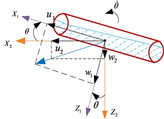
Let be the coordinate system obtained by translating the earth-fixed coordinate system parallel to itself until its origin coincides with the origin of the body-fixed coordinate system. Then, the coordinate system is rotated a yaw angle about the axis. This yields the coordinate system . The coordinate system is rotated a pitch angle about the axis. This yields the coordinate system . Finally, the coordinate system is rotated bank or roll angle about the axis. This yields the body-fixed coordinate system , shown on Fig. 2. Fig. 4 is shown the rotation sequence according to the -convention showing both the linear () and angular () velocities. The rotation sequence is written as:
From liquid in satisfy the continuity equation, meet in impermeable conditions, meeting the conditions of kinematics and dynamics in the , available control equations as follows:
In above type, for free surface wave height function; for the outward normal direction of wet surface of tank; for liquid particle diameter bolts relative point . When lateral excitation of tank is 0, liquid is freely sloshing. So on the type of boundary problem is transformed into a type Eq. (17). In above type, for liquid sloshing state function; for the wave height state function; for the freedom liquid sloshing characteristic frequency, Hz.
In that case, the kinematic equations can be described by two Euler angle representations with different singularities. Another possibility is to use a quaternion representation. This is the topic of the next section. Summarizing the results from this section, the kinematic equations can be expressed in vector form as:
The following coordinate transformation matrix for the Euler parameters:
The transformation relating the linear velocity vector in the inertial reference frame to the velocity in the body-fixed reference frame can be expressed as:
where with defined is the rotation matrix. Hence:
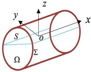
Fig. 4The rotation sequence according to the xyz-convention showing both the linear (u,v,w) and angular (p,q,r) velocities, boundary conditions. Ω is liquid domain, Σ is wet surface of tank, S is free surface
a) Rotation angle about ()
b) Rotation angle about ()
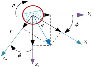
c) Rotation angle about ()
d) The boundary conditions
The angular velocity transformation can be derived by differentiating:
Let us define the matrix as:
where is a unique vector defined as the angular velocity of the body-fixed rotating frame with respect to the earth-fixed frame at time . Introducing the notation :
2.2.3. Newtonian and Lagrangian mechanics
The 6-DOF nonlinear dynamic equations of motion can be conveniently expressed as:
where: – inertia matrix (including added mass); – matrix of Coriolis and centripetal terms (including added mass); – damping matrix; – vector of gravitational forces and moments; – vector of control inputs.
Consider a body-fixed coordinate system rotating with an angular velocity about an earth-fixed coordinate system . Arbitrary body-fixed coordinate system with origin in the body-fixed frame is defined as:
where , and are the moments of inertia about the , and -axes and , and .
as the mass density of the body. Consequently, we can represent the inertia tensor in vectorial form as:
Another useful definition of is:
As Parallel Axes Theorem, the inertia tensor about an arbitrary origin is defined as:
, yields the following set of equations:
where:
Hence 6-DOF equation of motion:
The vectorial representation of the 6-DOF equations of motion:
where is the body-fixed linear and angular velocity vector and is a generalized vector of external forces and moments.
3. Experiment test
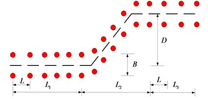
In order to verify the accuracy of the simulation results, the common tanker on the market is contrasted with the 6-DOF equation of motion. Real vehicle experiment adopts the single line test method, test pegged diagram as shown in Fig. 5. 6 m; 30 m; 25 m or 40.6 m (the value can be adjusted according to the specific models); Distance: a lane change 15 m. Benchmarking width: 1.20.25, for car width.
Fig. 5Pole layout diagram
The instantaneous maximum moments are contrasted by the real vehicle test and 6-DOF equation of motion (Fig. 6(a)). Two curves are the change tendency of the instantaneous maximum moments when the charging ratio from 40 % to 90 %. Both have the same change trend, which can verify the feasibility and applicability of the 6-DOF equation of motion.
Fig. 6Contrast test
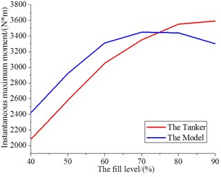
a) Instantaneous maximum moment of the tanker and the model
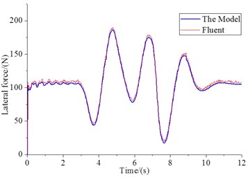
b) Lateral force of Fluent and the model
In the field of computational liquid dynamics, the determination of solving domain and the control equation of discretization is the key point. According to the difference principle and way of discrete, the common discretization method can be divided into: finite difference method, finite element method (FEM) and finite volume method (FVM). The FVM is the most widely used and FEM is relatively mature. We used the Fluent software to verify the 6-DOF equation of motion, to simulate on the lateral force of tanks. It can be seen under the lateral acceleration of the time-varying, the use of Fluent software and dynamic model for the liquid sloshing values coincide well (Fig. 6(b)).
According to the different filled level tank liquid by simulating, the coordinates of the mass centre to change with the force and moment about , , -axis. The related parameters in the simulation are listed as below, the friction coefficient is set as 0.5; the turning radius is 25 m; the truck mass is 5000 kg; the liquid mass is 4000 kg; suspension stiffness is 1000 kN/m; suspension damping is 15 kN/m; half track width is 2 m; half spring spacing is 3 m; the major axis and minor axis of ellipse are equal to 2.4 m and 1.8 m, respectively.
Fig. 7The moment under the filled level 20 %-50 %
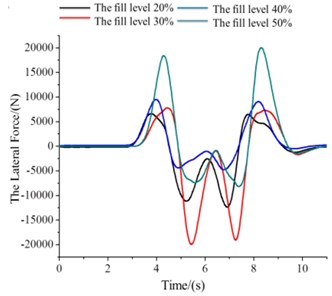
a) The values of (The force about -axis)
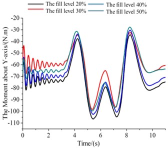
b) The values of (The moment about -axis)
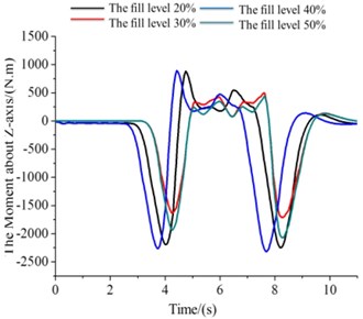
c) The values of (The moment about -axis)
1) , the filled level is 20 to 50 %, and .
The numerical simulations are used for 20% to 50% filled level of the tank. Excitation parameters are that the left front and left rear wheel are the sine functions, the right front and right rear wheel are the cosine function. Fig. 7 shows the force about -axis. Fig. 7(b), (c) are shown the moments about -axis and -axis.
2) , the filled level is 50 % to 100 %.
Due to the liquid mass center equation about liquid filled level 0-50 % and the equation of 50-100 % are different, that draw the following series of graphics (Fig. 8(a)-(c)). Fig. 9(a) shows the force about the -axis. Fig. 8(b), (c) is shown the moments about -axis and -axis.
4. Discussion
To solve the partially-filled tank truck liquid sloshing dynamics, this study established tank of liquid C.G. motion equation. Moreover, six degrees of freedom nonlinear liquid sloshing model were established by applying the Euler transform ideas. Finally, two sets of equations are coupled by using MATLAB ODE to simulate.
1) , the filled level is 0 to 50 %:
At the beginning, the lateral force of four different situations is basically the same they were slowly rising trend (Fig. 7(a)). After 2.5 s, the lateral force of 0.4 (the filled level 40 %) is higher than other three situations. Then, 0.3 for the liquid level is the smallest in the lateral force. At the same time it has been at a lower level, which accords with the actual situation.
The moment of different filled level related to the -axis is increased at the simulation phase (right-hand rule) (Fig. 7(b)). Four kinds of situations are presented slowly rising trend. But 0.5 corresponding moment value is slightly larger than others. Four kinds of filled level of the yawing moment are equal that is the first time (at 1.8 s). In the process of the whole simulation, four equal yawing moments appear many times. In the process of the whole simulation, the corresponding moment value about 0.5 is faster than others growth or decline, took two of local minimum or maximum on the four levels.
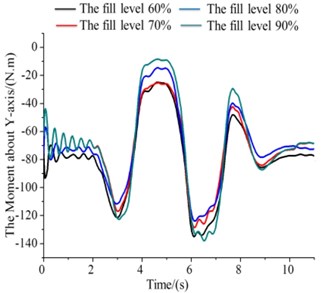
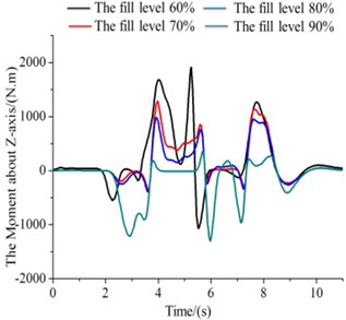
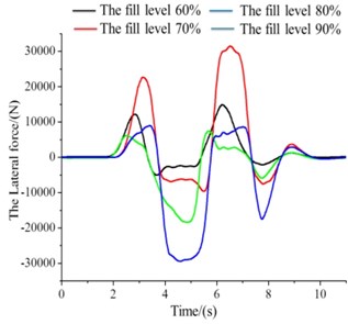
Fig. 8The moment under the filled level 60 %-90 %
a) The values of (The force about -axis)
b) The values of (The moment about -axis)
c) The values of (The moment about -axis)
The four different liquid level corresponding moment’s absolute values were in a state of rise about the rotational moment of the axis (Fig. 7(c)). After the start of about 1 s, four in moments of liquid level are equal to that of the latter continue to rise. Then, the 0.5 corresponding moment value rises faster, always maintain a high state.
2) , the filled level is 50 % to 100 %:
The tank of liquid sloshing numerical simulation results for the filled level 50 % to 90 % as shown Fig. 8(a)-(c). The shape of the graphic below is some similar, but there are differences in values. In Fig. 8(a), when simulation to 2.5 seconds, four different lateral force all showed a trend of rise, but the corresponding force about 0.9 rose slowly. It demonstrates that, the mass centre of high liquid filled level relatively small variations, the lateral force is small in the process of liquid sloshing. As is Fig. 8(b), 0.6 corresponding moment decreased rapidly and reach the maximum points. In addition, Roll moment curve about 0.9 (the filled level 90 %) is more gentle, has good ability to resist roll. In Fig. 8(c), about the rotational moment of the axis in the filled level from 50 % to 90 %, the four different liquid level corresponding moment’s absolute values were in a state of rise. After the start of about 1 s, moments of several liquid filled levels are equal to that of the latter continue to rise. In the meantime, the 0.9 corresponding moment value rises faster and always maintain a high state.
5. Conclusion
The quality of the tank liquid will increase with the increase of liquid ratio. Its mass center height increases, the external incentives for the same, the tank lateral sloshing larger than the small ones. The more liquid tank is mass center height increase at the same time.
In the case of liquid ratio is less than 50 %, the roll, yawing and pitching moment smaller than others. But in the case of liquid ratio is more than 50 %, three axis force and moment obvious different. Because the free surface is small, high liquid filled levels in the center of mass of liquid tank is relatively small variations, received the lateral force is small, but quite a few requirements of speed. Also, 0.9 (90 %) for the liquid level of the roll torque curve is more gentle, has good ability to resist lateral tilt.
This work in view of the friction coefficient is 0.5, the turning speed of is 80 km/h, turning radius of is 25 m, elliptical tank truck coupled simulation analysis, the model better reflects the external excitation caused by the sloshing of the tank of liquid sloshing in the tank. It provides a theoretical basis for further study on the different surface friction coefficient, turning speed and turning radius of the various cross section shape and size of the liquid tank design.
References
-
Daniel J., Chien S. Identifying Factors and Mitigation Technologies in Truck Crashes in New Jersey. Final Report 09, 2003.
-
Douglas B. P., Kate H., Nancy M., et al. Cargo Tank Roll Stability Study. Final Report GS23-0011L, 2007.
-
Wang W. H., Cao Q., Ikeuchi K., Bubb H. Reliability and safety analysis methodology for identification of drivers’ erroneous actions. International Journal of Automotive Technology, Vol. 11, Issue 6, 2010, p. 873-881.
-
Wang W., Zhang W., Guo H., Bubb H., Ikeuchi K. A safety-based approaching behavior model with various driving characteristics. Transportation Research Part C, Vol. 19, Issue 6, 2011, p. 1202-1214.
-
Kang X., Rakheja S., Stiharu I. Optimal tank geometry to enhance static roll stability of partially filled tank vehicles. SAE Paper No. 1999-01-3730, 1999, p. 542-553.
-
Romero J. A., Ramírez O., Fortanell J. M., Martínez M., Lozano A. Analysis of lateral sloshing forces within road containers with high fill levels. Journal of Automobile Engineering, Proceedings of the Institution of Mechanical Engineers, Part D, Vol. 220, Issue 3, 2006, p. 303-312.
-
Ranganathan R., Rakheja S., Sankar S. Steady turning stability of partially filled tank vehicles with arbitrary tank geometry. Journal of Dynamic Systems, Measurement and Control, Transactions of the ASME, Vol. 111, Issue 3, 1989, p. 481-489.
-
Popov G., Sankar S., Sankar T. S., Vatistas G. H. Dynamics of liquid sloshing in horizontal cylindrical road containers. Proceedings of the Institution of Mechanical Engineers, Part C, Vol. 207, Issue 6, 1993, p. 399-406.
-
Toumi M., Bouazara M., Richard M. J. Impact of liquid sloshing on the behaviour of vehicles carrying liquid cargo. European Journal of Mechanics, A, Vol. 28, Issue 5, 2009, p. 1026-1034.
-
Thor Fossen I. Guidance and Control of Ocean Vehicles. 1995.
-
Romero J. A., Lozano A., Ortiz W. Modeling of liquid cargo–vehicle interaction during turning manoeuvres. 12thIF To MM World Congress, Besançon, 2007.
-
Kolaei A., Rakheja S., Richard M. J. Range of applicability of the linear fluid slosh theory for predicting transient lateral slosh and roll stability of tank vehicles. Journal of Sound and Vibration, Vol. 333, Issue 1, 2014, p. 263-282.
-
Kolaei A., Rakheja S., Richard M. J. Effects of tank cross-section on dynamic fluid slosh loads and roll stability of a partly-filled tank truck. European Journal of Mechanics-B/Fluids, Vol. 46, 2014, p. 46-58.
-
Hughes P. C. Spacecraft Attitude Dynamics. John Wiley and Sons, NY, 1986.
-
Kane T. R., Likins P. W., Levinson D. A. Spacecraft Dynamics. McGraw-Hill, NY, 1983.
About this article
This work is supported by the National Science Foundation of China (Grant No. 51375200).
