Diagnostics of gear faults using ensemble empirical mode decomposition, hybrid binary bat algorithm and machine learning algorithms

Rajeswari, C.; Sathiyabhama, B.; Devendiran, S.; Manivannan, K.

Journal of Vibroengineering

Browse Journal

Submit article

Published: 15 May 2015

Check for updates

Diagnostics of gear faults using ensemble empirical mode decomposition, hybrid binary bat algorithm and machine learning algorithms

C. Rajeswari¹

B. Sathiyabhama²

S. Devendiran³

K. Manivannan⁴

¹Research Scholar, Faculty of Information and Communication Engineering, Anna University, Chennai, Tamil Nadu, India

²Department of Computer Science and Engineering, Sona College of Technology, Salem, Tamil Nadu, India

^{3, 4}School of Mechanical and Building Sciences, VIT University, Vellore, Tamil Nadu, India

Corresponding Author:

C. Rajeswari

Cite the article Download PDF

Downloads 1366

WoS Core Citations 8

Abstract

Early fault detection is a challenge in gear fault diagnosis. In particular, efficient feature extraction and feature selection is a key issue to automatic condition monitoring and fault diagnosis processes. In order to focus on those issues, this paper presents a study that uses ensemble empirical mode decomposition (EEMD) to extract features and hybrid binary bat algorithm (HBBA) hybridized with machine learning algorithm to reduce the dimensionality as well to select the predominant features which contains the necessary discriminative information. Efficiency of the approaches are evaluated using standard classification metrics such as Nearest neighbours, C4.5, DTNB, K star and JRip. The gear fault experiments were conducted, acquired the vibration signals for different gear states such as normal, frosting, pitting and crack, under constant motor speed and constant load. The proposed method is applied to identify the different gear faults at early stage and the results demonstrate its effectiveness.

1. Introduction

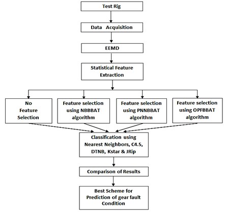
Gears are used almost in all power transmission systems in variety of applications and it is one of the most significant and frequently encountered components in rotating machinery. Gear health condition is directly propotional to the performance of the machinery. Thus gear fault diagnosis has received intensive study for several dacades [1]. One of the principal method for gear fault diagnosis is vibration analysis [2]. It gives more information about the operational conditions of the machinery component through vibration signature. Three main categories of waveform data analysis are used in vibration based condition monitoring: time-domain analysis, frequency-domain analysis and time-frequency analysis. Time-domain analysis is directly based on the time waveform itself. Traditional time-domain analysis calculates characteristic features from time waveform signals as descriptive statistics such as peak, peak to-peak interval, mean, standard deviation, crest factor and high-order statistics: skewness, kurtosis, root mean square. These features are usually called time-domain features [3]. Frequency-domain analysis is based on the transformed signal in frequency domain. The main advantage is, it has an ability to easily identify and isolate certain frequency components of interest. The most widely used conventional analysis is the spectrum analysis by means of fast Fourier transform (FFT). The main idea of spectrum analysis is to look at the whole spectrum or at certain frequency components of interest and thus extract features from the signal [4]. One limitation of frequency-domain analysis is, its inability to analyse non-stationary waveform signals generated when machinery faults occur. To overcome this problem, time-frequency analysis, which investigates waveform signals in both time and frequency domain, has been developed. Traditional time–frequency analysis uses time-frequency distributions, which represent the energy or power of waveform signals in two-dimensional functions of both time and frequency to reveal better the fault patterns for more accurate diagnostics. Short-time Fourier transform (STFT) or spectrogram (the power of STFT) [5] and Wigner-Ville distribution [6] are the most popular time-frequency distributions. Another transform is the wavelet transform (WT), which is a time-scale representation of a signal. WT has an ability to produce, a high frequency resolution at low frequencies, and a high time resolution at high frequencies, for signals with long duration low frequencies and short duration high frequencies as well used to reduce noise in raw signals. WT has been successfully applied in fault diagnostics of gears [7], bearings [8] and other mechanical systems [9]. Empirical Mode Decomposition (EMD) has attracted attention in recent years due to its ability to self-adaptive decomposition of non-stationary signals and EMD confirm its effective application in many diagnostic tasks [10]. Manually analysing the vibration data for large equipment with large collected data is tedious. Hence, the need to automatically analyze the data is necessary and computational intelligence models have a significant impact on fault diagnosis research that implements feature extraction, feature optimization and classification. Many of the artificial intelligence techniques are deployed so far in fault diagnosis such as artificial neural networks (ANNs) [11], support vector machines (SVMs) [12] and K-nearest neighbor (KNN) method [13] and so on and achieved satisfactory diagnosis accuracy. In intelligent fault diagnosis method, statistical characteristics were calculated after signal processing and it has vast number of features with variety of domains which poses challenges to data mining. In order to achieve successful classification process in terms of prediction accuracy, feature selection is consider essential. Feature selection methods such as principal component analysis (PCA) [14], Genetic algorithm (GA) [15] and J48 algorithm [16] are widely used to decrease dimensions of features. In the present study, EEMD is a preprocessing method used to extract more useful fault information from the gear vibration signals. The proposed methodology, is made up of following parts, gear experiment, data acquisition from test rig, signal preprocessing, feature selection, classification and final condition identification.The methodology of the present work is illustrated in the Fig. 1. In Section 1 we briefly reviewed the works which are strictly connected to the subject of this paper. In Section 2 illustrates briefly about theoretical background of EEMD and statistical feature extraction. Section 3 briefs about the feature selection algorithm such as HBBAT and its methodologies. Section 4 explains briefly about classification algorithms. In Section 5 experimental setup and experimental procedure is presented. In Section 6 Analysis of simulated data according to the presented procedure is discussed. In Section 7 the results for the same is presented and final section contains conclusions.

Fig. 1Methodology

2. Theoretical background of EEMD

The empirical mode decomposition (EMD) is a non-linear, multi- resolution and self-adaptive decomposition technique. It offers a different approach to signal processing and it is not defined as integral transformation but is rather an empirical algorithm based method. EMD can adaptively decompose a complicated signal into a set intrinsic mode functions (IMFs), without preliminary knowledge of the nature and the number of IMF components embedded in the data. IMF function satisfies the following two conditions: (1) in the whole data set, the number of extrema and the number of zero-crossings must be either equal or differ at most by one, (2) at any point, the mean value of the envelope defined by local maxima and the envelope defined by the local minima is zero.

Fig. 2Flow chart of EEMD

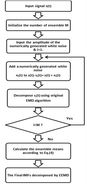
Table 1Pseudo code of EEMD algorithm

Algorithm: EEMD

Input: Input signal

s (t)

Output: Final IMF decomposed by EEMD

Step 1: Initialize the number of ensemble ‘

M

’

Step 2: Input the amplitude of the numerically generated white noise and

i = 1.

Step 3: Add a numerically generated white noise

n (t)

with the given amplitude to the original signal to generate a new signal:

s_{i} (t) = s (t) + n_{i} (t),

where

n_{i} (t)

denotes the

i

th added white noise series and represents the noise-added signal of the

i

-th trial, while

i =

1, 2,...,

M

.

Step 4: Use the original EMD algorithm to decompose the newly generated signal

s_{i} (t)

into IMFs:

s_{i} (t) = \sum_{x = 1}^{x} I M F_{i, x} (t) + r_{i, x} (t),

where ‘

x

’ is the number of IMFs,

r_{i, x} (t)

is the final residue, which is the mean trend of the signal, and

I M F_{i, x} (t)

represents the IMFs:

(I M F_{i, 1}, I M F_{i, 2}, I M F_{i, 3}, \dots, I M F_{i, x}),

which include different frequency bands ranging from high to low.

Step 5: Repeat steps 3 and 4 ‘

M

’ times with a different white noise series each time to obtain an ensemble of IMFs:

[\{I M F_{1, x} (t), I M {F_{2}}_{, x} (t), I M {F_{3}}_{, x} (t), \dots, I M F_{M, x} (t)\}],

where,

x =

1, 2,...,

X

.

Step 6: Calculate the ensemble means of the corresponding IMFs of the decomposition as the final result:

I M F_{x} (t) = \sum_{i = 1}^{M} I M F_{i, x} (t),

where

I M F_{x} (t)

is the

x

th IMF decomposed by EEMD, while

i =

1, 2,…,

M

and

x =

1, 2,…,

X

.

The fact that the signal is decomposed without a preset basis function and the level of decomposition is self-adaptively determined by the nature of decomposed signal is often reported as the main advantage of EMD against widely used wavelet based techniques [17]. However, EMD still agonize from the mode mixing problem. Mode mixing is defined as a single IMF including oscillations of dramatically disparate scales, or a component of a similar scale residing in different IMFs. It is a result of signal intermittency [18], which cause serious aliasing in the time–frequency distribution and make individual IMF unclear. To overcome the drawback of the mode mixing, an effective noise-assisted method named EEMD [19] which significantly reduces the chance of undue mode mixing and preserves the dyadic property of the decomposition for any data. EEMD is an improved version of original EMD and a more mature tool for a non-linear and non-stationary signal processing techniques. The principle of the EEMD is simple: the added white noise populates the whole time-frequency space uniformly, facilitating a natural separation of the frequency scales, which reduces the occurrence of mode mixing. The flow chart of EEMD algorithm is depicted in Fig. 2 and its pseudocode is in Table 1.

Table 2Statistical features

Time domain features
$T f_{i} = \frac{\sum_{n = 1}^{N} y (n)}{N}$	$T f_{7} = m a x (y (n))$	$T f_{13} = \frac{(T f_{7})}{(T f_{4})}$
$T f_{2} = \sqrt{\frac{\sum_{n = 1}^{N} (y (n))^{2}}{N}}$	$T f_{8} = m i n (y (n))$	$T f_{14} = \frac{(T f_{7})}{(T f_{3})}$
$T f_{3} = {(\frac{\sum_{n = 1}^{N} \sqrt{\|y (n)\|}}{N})}^{2}$	$T f_{9} = T f_{7} - T f_{8}$	$T f_{15} = \frac{(T f_{5})}{(T f_{2})^{3}}$
$T f_{4} = \frac{\sum_{n = 1}^{N} \|y (n)\|}{N}$	$T f_{10} = \frac{\sum_{n = 1}^{N} (y (n) - T f_{1})^{2}}{N - 1}$	$T f_{16} = \frac{(T f_{6})}{(T f_{2})^{4}}$
$T f_{5} = \frac{\sum_{n = 1}^{N} (y (n) - T f_{1})^{3}}{N}$	$T f_{11} = \frac{(T f_{2})}{(T f_{4})}$
$T f_{6} = \frac{\sum_{n = 1}^{N} (y (n) - T f_{1})^{4}}{N}$	$T f_{12} = \frac{(T f_{7})}{(T f_{2})}$
Frequency domain features
$F f_{i} = \frac{\sum_{k = 1}^{K} z (k)}{K}$	$F f_{7} = \sqrt{\frac{\sum_{k = 1}^{K} F_{k}^{2} z (k)}{\sum_{k = 1}^{K} z (k)}}$	$F f_{13} = \frac{\sum_{k = 1}^{K} (F_{k} - F f_{5})^{1 / 2} z (k)}{K \sqrt{F f_{6}}}$
$F f_{2} = \frac{\sum_{k = 1}^{K} (z (k) - F f_{1})^{2}}{K - 1}$	$F f_{8} = \sqrt{\frac{\sum_{k = 1}^{K} F_{k}^{4} z (k)}{\sum_{k = 1}^{K} F_{k}^{2} z (k)}}$
$F f_{3} = \frac{\sum_{k = 1}^{K} (z (k) - F f_{1})^{3}}{K {(\sqrt{F f_{2}})}^{3}}$	$F f_{9} = \frac{\sum_{k = 1}^{K} F_{k}^{2} z (k)}{\sqrt{\sum_{k = 1}^{K} z (k) \sum_{k = 1}^{K} F_{k}^{4} z (k)}}$
$F f_{4} = \frac{\sum_{k = 1}^{K} (z (k) - F f_{1})^{4}}{K {(\sqrt{F f_{2}})}^{2}}$	$F f_{10} = \frac{(F f_{5})}{(F f_{6})}$
$F f_{5} = \sqrt{\frac{\sum_{k = 1}^{K} (F_{k} - F f_{5})^{2} z (k)}{K}}$	$F f_{11} = \frac{\sum_{k = 1}^{K} (F_{k} - F f_{5})^{3} z (k)}{K {(F f_{6})}^{3}}$
$F f_{6} = \frac{\sum_{k = 1}^{K} F_{k} z (k)}{\sum_{k = 1}^{K} z (k)}$	$F f_{12} = \frac{\sum_{k = 1}^{K} (F_{k} - F f_{5})^{4} z (k)}{K {(F f_{6})}^{4}}$

2.1. Statistical feature extraction

Statistical feature extraction is an important step in machine fault diagnosis. When the gear fault occurs due to non-stationary signal variation, amplitude, time domain and frequency spectrum distribution of fault gear may be different from those of normal gear and also it creates the newfrequency components. Twenty-nine feature parameters are listed in Table 2. 16 features indicate the time-domain statistical characteristics, and remaining 13 features indicate frequency-domain statistical characteristics. Feature ${T f}_{1}$ – ${T f}_{10}$ gives the time domain vibration amplitude and energy. Feature ${T f}_{11}$ – ${T f}_{16}$ gives the time series distribution of same domain. Feature ${F f}_{1}$ gives the information about frequency domain energy. Convergence of the spectrum power may described by Feature ${F f}_{2}$ – ${F f}_{5}$ . Position change of the main frequencies described by ${F f}_{6}$ – ${F f}_{9}$ [20].

3. Feature selection using Hybridized binary bat algorithm

The proposed methodology primarily concentrates on representing each bat with a binary vector, which corresponds that a feature will be selected or not to construct the new dataset. The quality of the solution is provided by building a classifier using the encoded bats with the selected features and also to classify the evaluating set. Thus, we require classifiers which builds the classification model faster and accurate. The cost function to be maximised is the classification accuracy obtained from the classifiers among: Optimal Path Forest (OPF), Naive Bayes (NB), Probabilistic Neural Network (PNN).

3.1. Binary bat algorithm

The preying nature of bats is interesting as it uses echolocation that has drawn attention of many researchers to solve optimization problems. The idea behind echolocation of bats is that, the bat emits a loud and short pulse of sound which gets reflected and reaches the bat, based on the reflected sound the bat determines the type of the object and its proximity. Based on the behaviour of the bats, a new meta heuristic optimization technique called Bat algorithm [21] were developed and in order to model this algorithm some rules has to be idealized, as follows:

1) All bats uses the idea of echolocation to determine the prey and its proximity.

2) Every bat $B_{i}$ requires velocity ${v e l}_{i}$ to fly randomly at position ${p o s}_{i}$ with a frequency ${f r e q}_{l o w}$ , varying wavelength $λ$ and loudness $L_{0}$ to search its prey. The rate of pulse emission $p$ can vary between 0 and 1 based on the distance of their prey.

3) Loudness varies from $L_{0}$ to a minimum $L_{m i n}$ .

The initial position ${p o s}_{i}$ , ${v e l}_{i}$ and frequency ${f r e q}_{i}$ are initialized and updated for each bat at each iteration $i t e r$ until it reaches the maximum number $I$ as follows:

1

{f r e q}_{i} = f_{l o w} + (f_{h i g h} - f_{l o w}) β B_{i},

2

{v e l}_{i}^{n} (i t e r) = {v e l}_{i}^{n} (i t e r - 1) + [{\hat{p o s}}^{n} - {p o s}_{i}^{n} (i t e r - 1)] {f r e q}_{i},

3

{p o s}_{i}^{n} (i t e r) = {p o s}_{i}^{n} (i t e r - 1) + {v e l}_{i}^{n} (i t e r),

where $β$ is a randomly generated number within [0, 1]. ${p o s}_{i}^{n} (i t e r)$ denotes the value of the decision variable $n$ for bat $i$ at time step $i t e r$ . The results of ${f r e q}_{i}$ is used to control the movements of bats. The variable ${\hat{p o s}}^{n}$ represents the current global best solution for the decision variable $n$ by comparing the solutions of $B$ bats. The diversity of the possible solutions are increased by employing a random walk through which a solution is selected among the best solutions and a local solution is generated around the best solution using the Eq. (4):

4

{p o s}_{i}^{n} (o l d) = {p o s}_{i}^{n} (n e w) + ϵ \bar{L} (i t e r),

in which $\bar{L} (i t e r)$ denotes the average loudness of all bats at time $i t e r$ and $ϵ$ denotes the direction and strength of the random walk. This proposed methodology is concerned about selecting or deselecting a feature, so in the algorithm the bats position is restricted to binary values using sigmoid function and hence the Eq. (3) could be replaced by:

5

{p o s}_{i}^{n} (i t e r) = \{\begin{matrix} 1, & f S i g ({v e l}_{i}^{n}) > σ, \\ 0, & o t h e r w i s e, \end{matrix}

6

S i g ({v e l}_{i}^{n}) = \frac{1}{1 + e^{- {v e l}_{i}^{n}}},

at each step of iteration $i t e r$ the loudness $L$ and pulse rate $p$ are updated as follows:

7

L_{i} (i t e r + 1) = α L_{i} (i t e r),

8

p_{i} (i t e r + 1) = p_{i} (0) [1 - \exp (- γ i t e r)],

where $α$ and $γ$ are adhoc constants. The pulse rate $p_{i} (0) \in [0, 1]$ . The step by step procedure of the hybridized binary bat algorithm is given in Table 3.

Table 3Pseudo code of hybridized binary bat algorithm

Algorithm: Hybridized Binary Bat algorithm

Input:

T_{1}

– Labeled Unreduced feature set;

T_{2}

– Unlabeled Unreduced feature set;

B

– population size;

F

– Number of features;

I t e r

– Number of iterations;

L

– Loudness;

p

,

ϵ

,

α

,

γ

– pulse emission rate.

Output: reduced feature set.

1) For each

{B a t}_{i} (\forall i = 1, \dots, B)

, do

2) For each feature

n (\forall n = 1, \dots, F)

; do

{p o s}_{i}^{n} \leftarrow r a n d o m \{0, 1\}

;

3)

V_{i}^{n} \leftarrow 0

;

L_{i} \leftarrow r a n d o m {1, 2}

;

p_{i} \leftarrow r a n d o m {0, 1}

;

{f i t n e s s}_{i} \leftarrow - \infty

;

4)

G_{f i t} \leftarrow - \infty

;

5) for each iteration

I t e r

,

(I t e r = 1, \dots I)

, do

6) for each bat

{B a t}_{i} (\forall i = 1 \dots B)

, do

7) create

T_{1}^{'}

and

T_{2}^{'}

from

T_{1}

and

T_{2}

respectively such that both contains only features in

{B a t}_{i}

in which

{p o s}_{i}^{n} \neq 0

;

\forall n = 1, \dots, F

.

8) Select among OPF, NB,PNN; train the selected classifier over

T_{1}^{'}

, evaluate over

T_{2}^{'}

and stores accuracy of the respective classifier in A.

9)

r_{d} \leftarrow r a n d o m \{0, 1\}

10) If

(r_{d} < L_{i}

and

A > {f i t n e s s}_{i})

, then

11)

{f i t n e s s}_{i} \leftarrow A

;

L_{i} \leftarrow α L_{i}

;

p_{i} \leftarrow p_{i} [1 - \exp (- γ I t e r)]

12) [

M_{f}, M_{I}] \leftarrow m a x (f i t n e s s)

13) If

(M_{f} > G_{f})

then

G_{f} \leftarrow M_{f}

14) For each dimension

n (\forall n = 1, \dots, B)

, do

15)

{\hat{p o s}}^{n} \leftarrow {\hat{p o s}}_{M I}^{n}

16) For each bat

{B a t}_{i} (\forall i = 1, \dots, B)

, do

β \leftarrow r a n d o m \{0, 1\}

;

r_{d} \leftarrow r a n d o m {0, 1}

17) If

{(r}_{d} > p_{i})

18) For each feature

n

(\forall n = 1, \dots, F)

do

19)

{p o s}_{i}^{n} = {p o s}_{i}^{n} + \in \bar{L}

;

σ \leftarrow r a n d o m \{0, 1\};

20) If

(σ < 1 \frac{1}{1 + e^{- {p o s}_{i}^{n}}})

then

{p o s}_{i}^{n} \leftarrow 1

; else

{p o s}_{i}^{n} \leftarrow 0

;

21)

r_{d} \leftarrow r a n d o m {0, 1}

22) If (

(r_{d} < L_{i}

and

({f i t n e s s}_{i} < G_{f})

, then for each feature

n (\forall n = 1, \dots, F)

do

23)

{f r e q}_{i} \leftarrow {f r e q}_{l o w} + (f_{h i g h} - f_{l o w}) β

;

24)

{v e l}_{i}^{n} \leftarrow {v e l}_{i}^{n} + ({\hat{p o s}}^{n} - {p o s}_{i}^{n}) {f r e q}_{i}

;

25)

{p o s}_{i}^{n} \leftarrow {p o s}_{i}^{n} + {v e l}_{i}^{n}

;

σ \leftarrow r a n d o m {0, 1}

;

26) If

(σ < \frac{1}{1 + e^{- {p o s}_{i}^{n}}})

then

{p o s}_{i}^{n} \leftarrow 1

; else

{p o s}_{i}^{n} \leftarrow 0

;

27) For each feature

n

(\forall n = 1 \dots F)

do

28)

f_{s u b}^{n} \leftarrow {\hat{p o s}}^{n}

29) Return

f_{s u b}

.

In the proposed pseudocode the Lines 1-4 initializes the population of bats. The line 2 defines the bats position randomly among 0 or 1, as the work is concerned about selecting or not selecting the features (Binary Bat). Lines 7-8 uses a classification technique among Optimal Path Forest (OPF), Naive Bayes (NB), Probabilistic Neural Network (PNN) to build a classification model, evaluates it over the selected features and stores the results of the classification accuracy in A. Lines 10-13 evaluates the bats position and updates its function, position, velocity and frequency.

At each iterations the values of the loudness and pulse rate are updated based on the Eqs. (7) and (8). The max function outputs the index and the fitness value of the the bat that maximizes the fitness function. Lines 13-15 updates the global best solution by comparing the solutions of $B$ bats. The variability of the solutions are increased in lines 17-20. Lines 21-26 updates the frequency, velocity and position of the bats as described in the equations 1, 2 and 3 respectively. Finally, the reduced subset of features are selected in Lines 27-28 and returned in Line 29. The parameters used in the algorithm has been summarized with their assigned values in Table 4.

Table 4Parameters and values used in hybridized binary bat algorithm pseudo code

Parameter	Symbol	Value
Population size	$B$	80
Training data set	$T 1$	(60/100)∙80 $=$ 48
Testing data set	$T 2$	(40/100)∙40 $=$ 32
Input feature set	$F$	29
Number of iterations	iter	600
Loudness	$L$	[1, 2]
Pulse rate	$p$	[0, 1]
Reduced feature set	$f_{s u b}$	Resultant feature set
Fitness vector of the population B	fitness	$- \infty$
Classification accuracy	$A$	Classification accuracy: OPF, NB, PNN
Random vector	$r_{d}$	[0,1]
Global best position	$G_{f i t}$	$- \infty$
Random vector	$β$	[0,1]
Maximum frequency	$f_{h i g h}$	O[1] $=$ 1
Minimum frequency	$f_{l o w}$	0
Random vector	𝜖	[–1, 1]
Average loudness of all bats	$\bar{L}$	Auxiliary
Fitness value of the bat that maximizes the fitness function	$M_{f}$	Auxiliary
Index of the bat that maximizes the fitness function	$M_{I}$	Auxiliary
Velocity of the variable $j$ for bat $i$	$V_{i}^{n}$	0
Position of the variable $j$ for bat $i$	${p o s}_{i}^{n}$	{0, 1}

3.2. Optimum-Path Forest (OPF) based feature reduction

The OPF is a classifier which builds a partition graph for the given feature set. The OPF algorithm builds two models: a training model and a testing model. In the training model the partition of the graph is carried out by evaluating the optimum paths from selective samples (nodes) to the remaining samples. Once the model is build a sample from the test set is connected to all training samples. The distance $d (s, t)$ to all training nodes are computed and used to weight the edges. The maximum arc weight from each training node to the test sample is given by Eq. (9), Eq. (10):

9

f_{m a x} (s) = \{\begin{array}{l} 0, & s \in S, \\ + \infty, & otherwise, \end{array}

10

f_{m a x} (π (s, t)) = \max {f_{m a x} (π), d (s, t)} .

The training node with minimum path cost will be assigned to the test sample. The classification accuracy of the OPF classifier has been used as the fitness function of the proposed optimised feature reduction problem. For more information [22].

3.3. Naïve Bayes based feature reduction

Naïve Bayes classifiers are classical statistical classifiers which is based on “Bayes Theorem” that assumes the features are conditionally independent of each other. Let $X$ be a data sample and $H$ be hypothesis that the sample $X$ belongs to the class $C$ . In order to determine the probability that the hypothesis $H$ holds given the data sample $X$ , Bayes theorem is used and given as:

11

P (H| X) = \frac{P (X| H) P (H)}{P (X)},

where, $P (H| X)$ and $P (X / H)$ are the posterior probabilities and $P (H)$ and $P (X)$ are the priori probabilites. For example $X$ is a instance of the gear fault condition described by the features mean and standard deviation and $X$ has 1.5 and 0.9 respectively. Suppose that H is a hypothesis that the instance $X$ class value be normal. Then $P (H / X)$ reflects the probability that instance $X$ will have normal fault condition given that we know the instance‘s mean and standard deviation. Similarly, in $P (X / H)$ $X$ is conditioned on $H$ . That is, it is the probability that the instance $X$ , has mean and stanard deviation as 1.5 and 0.9 respectively, given that we know the gear fault condition as normal. $P (H)$ , is the priori probability of $H$ . Then $P (H)$ reflects the probability that any given instance of the gear fault condition will be normal regardless of mean and standard deviation. Similarly, $P (X)$ is the probability that a instance from the set of samples will have mean and standard deviation as 1.5 and 0.9 respectively. For detailed explanation refer [23].

3.4. Probabilistic neural network based feature reduction (PNN)

PNN is a feed forward neural network. PNN consists of an input layer, pattern layer, summation layer, and an output layer. On receiving the input vector from the input layer, neurons in the pattern layer computes the probability density function for classification purpose. For the sample $X$ for which class label is unknown, the neuron $X_{k}$ computes the output using the equation:

12

Ψ_{k} (X) = \frac{1}{{(2 π)}^{p / 2} σ^{p}} e \frac{- {‖X - X_{k}‖}^{2}}{{2 σ}^{2}},

where $p$ is the length of the vector $X$ , $σ$ is the smoothing parameter and $X_{k}$ is the $k$ th sample.

The maximum likelihood ratio of the sample $X$ being classified in to class $C_{i}$ is computed in the summation layer by summarizing and averaging the probability density functions for the $n_{i}$ samples in the $i$ population. For detailed explanation refer [24].

4. Theoretical background of classification algorithms

4.1. Classification through nearest neighbours

K-nearest neighbour classifiers are based on learning by analogy that is comparing a test sample with training samples that are similar to it. When given an unknown sample the K-nearest neighbour classifier searches the $K$ training samples that have closest proximity to the unknown sample. The proximity between the testing sample and training sample is defined by a distance measure called as Euclidean distance which is given in Eq. (13). For more information about nearest neighbour, see [25]:

13

d i s (X_{1}, X_{2}) = \sqrt{\sum_{i = 1}^{n} {(x_{1 i} - x_{2 i})}^{2}} .

4.2. Classification through C4.5 algorithm

C4.5 algorithm or possibly J48 algorithm is an extension of ID3 algorithm. It is based on greedy approach, in which decision trees are built in a top-down manner and the tree structure consists of internal and external nodes connected by branches. Branch is a chain of nodes from root to a leaf and each node represents a feature. The occurrence of an feature in a tree provides the information about the importance of the associated feature as explained in [26]. To generate a decision tree from the training samples the algorithm requires three input parameters: $T$ – the training samples assosiated with the class labels, feature list-specifies the list of features that describe the samples and feature selection measure-specifies the feature splitting criteria. The tree starts as a single node $n$ , denoting the training samples in $T$ . If the samples in $T$ are all same class then n becomes a leaf node with that class label, otherwise feature selection measure is called to determine splitting criteria of the samples in $T$ . Let $F$ be a feature with values $\{f_{1}, f_{2}, \dots, f_{x}\}$ then feature selection measure is done for three possible scenarios: $F$ is discrete-valued, continuous valued, discrete-valued and a binary tree. The decision tree is build using the same process recursively, until the termination condition is true.

4.3. Classification through decision Tree Naive Bayes

Decision Tree Naive Bayes (DTNB) is a hybrid classifier that comprises of decision table/naive bayes. At each point in the search, the algorithm evaluates the merit of dividing the attributes into two disjoint subsets: one for the decision table, the other for naive Bayes. A forward selection search is used, where at each step, selected attributes are modeled by naive Bayes and the remainder by the decision table, and all attributes are modelled by the decision table initially. At each step, the algorithm also considers dropping an attribute entirely from the model. For more information, see [27].

4.4. Classification through K-Star

K-Star classifier is a variant of Lazy algorithms. K-Star uses a entropy measure to transform an sample to another, by randomly choosing between possible transformations. Given a set of samples $s$ and a set of possible transformations $T$ , it will map $s : S \to S$ , that is a sample $(a)$ to another sample $(b)$ . Then $T^{*}$ consists of members that has unique mapping on $S$ , given in Eq. (14):

14

s (a) = s_{n} (s_{n - 1} (\dots s_{1} (a) \dots)),

where $s = s_{1}, \dots, s_{n}$ , the probability function on $T^{*}$ is given by $p$ . $P^{*}$ is defined as the probability of all possible paths between sample $(a)$ and sample $(b)$ and is given in Eq. (15), Eq. (16):

15

P^{*} (\frac{b}{a}) = \sum_{s \in p i : s (a) = b} P (s),

and hence the $K^{*}$ function is given as:

16

K^{*} (\frac{b}{a}) = - \log_{2} P^{*} (\frac{b}{a}) .

For more information, refer [28].

4.5. Classification through JRip

JRip is an optimized version of IREP. Ripper is superivised classifier where the training samples are partitioned in to growing set and pruning set. Rules are built until information gain is possible further. The built rules are then passed on the pruning set where the unnecessary terms are eliminated in order to maximize the following function:

17

f = \frac{p + (N - n)}{P + N},

where $p$ and $P$ are the positive samples covered by rule and prune set respectively, similarly $n$ and $N$ are the negative samples covered by rule and prune set respectively. For more information about the classifier, refer [29].

5. Experimental setup and data acquisition

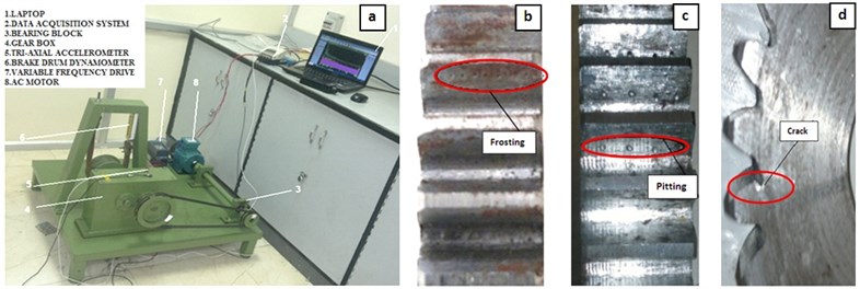
Fig. 3(a) shows the Test rig used in this work to verify the performance of the proposed method. The setup includes a gearbox, three phase 0.5 hp AC motor, variable frequency drive (VFD) for controlling the speed of the motor and allow the tested gear to operate under various speeds. A brake drum dynamometer setup has been connected to the gear box to control the load. Gearbox containing one pinion and one gear, connected to the motor by means of belt drive. SAE 40 oil is used as a lubricant in the gearbox. The gear used in the gear box is made of 045M15 steel, the spur gear has 36 teeth and pinion has 24 teeth. The spur gears used for this experiment have a module of 3 mm and a pressure angle of 20°. Four pinion gears with same specification and different conditions including one normal gear and three faulty gears such as normal gear, frost gear (Fig. 3(b)), pitted gear (Fig. 3(c)), crack gear (Fig. 3(d)) were fitted in the gear box with artificially created faults and are tested. Tri-axial accelerometer (Vibration sensor) with ±500 g sensitivity is fixed on top of the gearbox to measure the signals. The accelerometer sensor is connected to data acquisition system for acquiring the data. Here the rotational frequency of the pinion is set constant by maintaining the rotating speed and load, constantly.

Fig. 3Experimental setup and artificially induced gear failures

A digital signal processor dewesoft analyser (ATA0824DAQ51) and a laptop with the data acquisition software were used to collect the vibration data for further processing. During the test, rotation speed of the motor is 1000 rpm (16.67 Hz), the rotation speed of the gear is 11.11 Hz, and the mesh frequency is 522.24 Hz. The gear signals are extracted in the sampling rate of 12800 Hz (6400 data points per second). For 20 seconds 128000 data points were collected through accelerometer for each condition of gear. Even though the signals were collected tri-axially on the gearbox, the vibration signals of the vertical direction were more sensitive to the crack levels, they were considered and analysed in this paper. Each condition of gear signals are split into approximately 20 samples (each sample contains 6000 data points) and there are alltogether 80 data samples were collected.

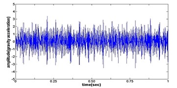
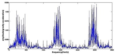
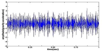
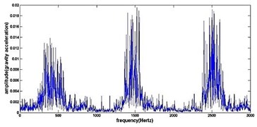
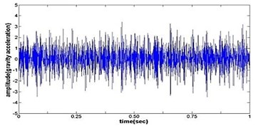
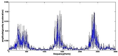
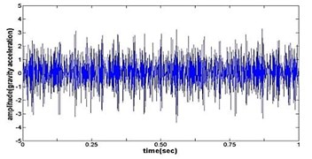
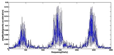
Fig. 4The original time domain signals and their corresponding spectrums of gear vibration signals in the four states of gear conditions

a) Time wave form of cracked gear

b) Frequency spectrum of cracked gear

c) Time wave form of frosting gear

d) Frequency spectrum of frosting gear

e) Time wave form of pitting gear

f) Frequency spectrum of pitting gear

g) Time wave form of normal gear

h) Frequency spectrum of normal gear

6. Intelligent fault diagnosis results and discussion

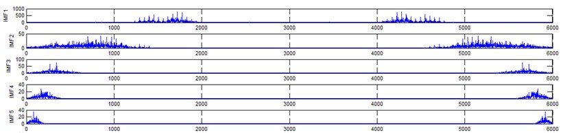
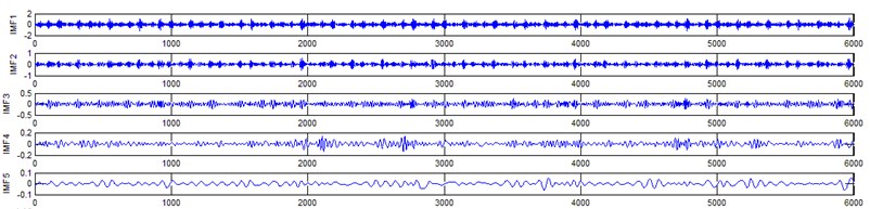
The vibration data acquired from the test rig of the gears are used to demonstrate the effectiveness of the proposed diagnosis method for the gear faults. The original time domain signals and their corresponding spectrums of gear vibration signals in the four states of gear conditions are given in Fig. 4(a) to (h). From both the time and frequency domain signals, direct categorization and differences among the four states of gears are understood and has great deal to identify the variation among them because of the noise present in the original signal of the four running conditions of gear. After then each vibration sample (original signal) was decomposed by EEMD. Initially in EEMD, two important parameters has to be set; the ensemble number $M$ and the amplitude of white noise $i$ . In general, an ensemble number of a few hundred will lead to a good result, and the remaining noise would cause negligible percent of error if the added noise has the standard deviation that is a fraction of the standard deviation of the input signal. For the standard deviation of the added white noise, it is suggested to be about 20 % of the standard deviation of the input signal [19]. Hence the two parameters of EEMD were set as $M =$ 100 and $i =$ 20 %. After setting the parameters, the signals were decomposed into ‘ $n$ ’ IMFs and one residue according to nature of the signal. For our case, IMF component decomposition identifies eleven modes: IMF 1-IMF 10 and one residue were arrived and depicted in Fig. 5(a) to Fig. 5(h). (IMF 6, IMF7, IMF8, IMF9, IMF10, and one residue (IMF11) is not shown in Figures for 3 faulty gear conditions) for four conditions of gear. The frequency spectrum is applied to each IMFs for four conditions of gear and it is depicted in the same Figure.

Fig. 5Gear signal EEMD results and their corresponding spectrums

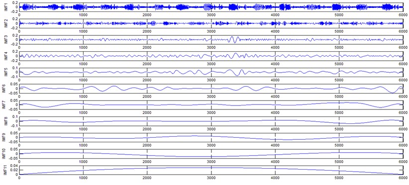
a) Normal gear signal EEMD results (upto 11 IMFS)

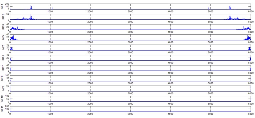
b) Corresponding spectrum of normal gear (EEMD) signal

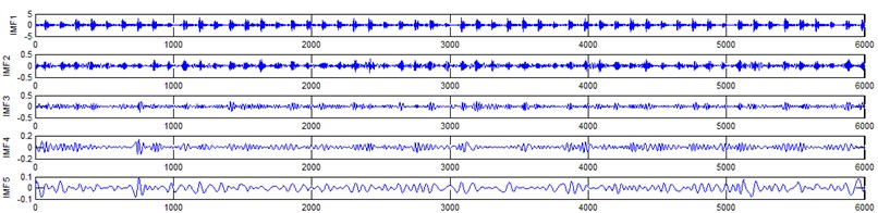
c) Crack gear signal EEMD results (upto 5 IMFS)

d) Corresponding spectrum of crack gear (EEMD) signal

e) Pitting gear signal EEMD results (upto 5 IMFS)

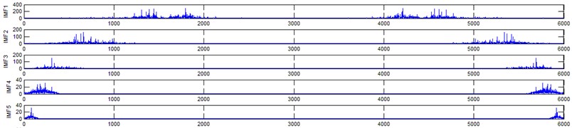
f) Corresponding spectrum of pitting gear (EEMD) signal

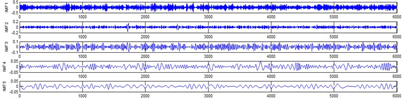
g) Frosting gear signal EEMD results (upto 5 IMFS)

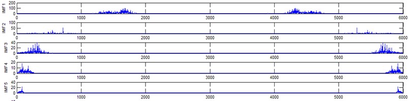
h) Corresponding spectrum of frosting gear (EEMD) signal

It represents the different frequency components excited by the different states of gear and IMF 11 is the residue, respectively. In the corresponding frequency spectrum of each IMFs say mode 1 (frequency spectrum of IMF1) contains the highest signal frequencies, mode 2 the next higher frequency band and so on. The vibration change caused by a localized damage at its early stage, is usually weak and contaminated by noise, so that early fault diagnosis is more difficult and needs more complicated methods. In the time domain, a localized gear fault causes amplitude and phase modulation of the gear meshing vibration which will not be deliberately seen many times; while in the frequency domain, these modulations appear as series of sidebands around the gear mesh frequency and its harmonics and this procedure was followed in the past decades. In automated fault diagnosis methodology, with the help of this knowledge, the informative features which are collected from the range of characteristic (gear mesh) frequencies will give more prediction accuracy. In this aspect the selection of IMFs for further processing is based on these criteria is as followed. From Fig. 5(b), we can know that the mode 1 (frequency spectrum of IMF1) is centered from 250 Hz to 1250 Hz, mode 2 (frequency spectrum of IMF2) with spectrum centered from 250 Hz to 750 Hz, mode 3 (frequency spectrum of IMF3) with spectrum centered from 0 Hz to 500 Hz and mode 4 (frequency spectrum of IMF4) with spectrum centered at 0 Hz to 250 Hz. Therefore, it is can be concluded that modes 1 to mode 2 accommodate the characteristic frequency (gear mesh frequency). Modes 7 and 8 are associated with the harmonic of the rotational frequency of the input shaft. For 2nd condition of gear (Fig. 5(d)) the mode 2 and mode 3 is centered on the range of 250 Hz to 1250 Hz, which can be obviously associated with the characteristic gear mesh frequency of the component. Similarly for 3rd (Fig. 5(f)) and 4th (Fig. 5(h)) condition also mode 2 lies or situated on the same range of values. From this inference it can be easily proven that the EEMD decomposes the vibration signal very effectively on an adaptive method. When compared to raw time and frequency signals, IMFs in both the domain are clearer even if it is hard to find the typical fault characteristics which can distinguish the four running conditions. Therefore the proposed intelligent based methodology is necessary to diagnose gear faults. Subsequently, 16-time domain and 13-frequency domain features are calculated only from IMF₁ to IMF₅ for each state of gear signal because of obvious characteristic and high signal energy present in first 4 IMFs. All the extracted features are normalized before given as input to the feature selection algorithms and classification process.

In order to reduce the dimensionality of the features classifier embedded binary bat algorithm is used for selecting the optimum features. Feature reduction process is carried out thrice using the three feature selection algorithms. In this present work,feature selection process are carried out using OPF, NB and PNN classifiers embedded with Binary Bat and the results of the selected feature‘s description and time taken for the process is depicted in the Table 5. The feature selection process were done in Matlab platform. The input features are catagorized into two types: Time and frequency domain features that are extracted from Time and frequency IMFs of EEMD and selected features from the same are separately fed input into weka embedded classifiers such as Nearest neighbours, C4.5, DTNB, K star and JRip to identify different states of gear through classification process. WEKA is an open source software issued under General Public License [30] used for classification process.

Table 5Feature selection results

Sl. No	Feature selection method	No. of features	Feature description	Run time (in sec)
1	No feature selection	All 29	${T f}_{1}$ – $T f_{16}$ and $F f_{1}$ – $F f_{9}$	0.1961
2	NBBBAT algorithm	10	$T f_{3}$ , $T f_{4}$ , $T f_{9}$ , $T f_{10}$ , $T f_{13}$ , $T f_{15}$ , $T f_{16}$ , $F f_{2}$ _, $F f_{4}$ , $F f_{7}$	0.1288
3	PNNBBAT algorithm	11	$T f_{3}$ , $T f_{5}$ , $T f_{9}$ , $T f_{11}$ , $T f_{13}$ , $T f_{15}$ , $F f_{1}$ , $F f_{3}$ _, $F f_{4}$ , $F f_{8}$ _, $F f_{8}$	0.1764
4	OPFBBAT algorithm	17	$T f_{1}$ , $T f_{2}$ , $T f_{3}$ , $T f_{5}$ , $T f_{9}$ , $T f_{11}$ , $T f_{13}$ , $T f_{14}$ , $T f_{15}$ , $T f_{16}$ , $F f_{1}$ , $F f_{2}$ , $F f_{3}$ _, $F f_{4}$ , $F f_{5}$ , $F f_{7}$ _, $F f_{9}$	0.1904

To measure and investigate the performance of the classification algorithms 75 % data is used for training and the remaining 25 % for testing purpose. The results of the simulation are shown in Tables 6 and 7. Table 6 summarizes the results based on accuracy and time taken for each simulation. Meanwhile, Table 7 shows the results based on error during the simulation. Figs. 6 and 7 shows the graphical representations of the simulation results. Based on the result (Table 6) it can be clearly noted that the highest accuracy is 93.4 % and the lowest is 72.2 %. The other schemes yields an accuracy between these two values. In fact, the highest accuracy belongs to the scheme –16, OPF BBAT hybridized with Nearest neighbour classifier and followed by scheme-6, Naivebayes BBAT hybridized with Nearest neighbour classifier and so on. The total time required to build the classification model (shown in Table 6) is also a crucial parameter in comparing the feature selection processes.

Table 6Simulation result of each scheme

Feature selection algorithm	Scheme title	Classification algorithm	Correctly classified instances in %	Incorrectly classified instances in %	Run time (sec)	Kappa statistic
No feature selection	Scheme-1	Nearest neighbour	85.4143	14.5857	0.29	0.7687
	Scheme-2	C4.5	83.7265	16.2735	0.87	0.7535
	Scheme-3	DTNB	77.1951	22.8049	0.52	0.6948
	Scheme-4	K star	84.7186	15.2814	0.23	0.7625
	Scheme-5	JRip	80.2675	19.7325	0.78	0.7224
NBBBAT	Scheme-6	Nearest neighbour	92.476	7.524	0.31	0.8323
	Scheme-7	C4.5	86.1596	13.8404	0.46	0.7754
	Scheme-8	DTNB	84.3351	15.6649	0.51	0.7590
	Scheme-9	K star	76.5433	23.4567	0.22	0.6889
	Scheme-10	JRip	75.4389	24.5611	0.76	0.6790
PNNBBAT	Scheme-11	Nearest neighbour	90.8041	9.1959	0.26	0.8172
	Scheme-12	C4.5	84.1435	15.8565	0.43	0.7573
	Scheme-13	DTNB	82.8353	17.1647	0.47	0.7455
	Scheme-14	K star	80.4826	19.5174	0.21	0.7243
	Scheme-15	JRip	79.5401	20.4599	0.71	0.7159
OPFBBAT	Scheme-16	Nearest neighbour	93.4001	6.5999	0.31	0.8406
	Scheme-17	C4.5	80.4639	19.5361	0.51	0.7242
	Scheme-18	DTNB	79.8002	20.1998	0.56	0.7182
	Scheme-19	K star	75.1502	24.8498	0.25	0.6764
	Scheme-20	JRip	72.2233	27.7767	0.84	0.6500

Fig. 6Comparison between feature selection method Vs Classifier accuracy

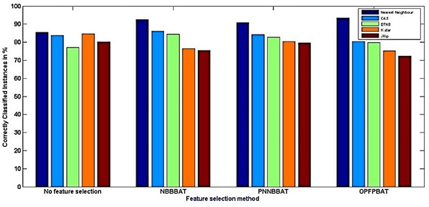
In this experiment, it is noted that a NBBBAT requires the shortest time which is around 0.1288 seconds compared to the others. OPFBBAT algorithm requires the largest model building time which is around 0.1904 seconds. In classification process K star classifier requires the shortest time which is around 0.21 seconds compared to the others. C4.5 algorithm requires the largest model building time which is around 0.87 seconds. One of the significant parameter, Kappa statistics is used to assess the accuracy. It is usual to distinguish between the reliability of the data collected and their validity.

Fig. 7Comparison between evaluation parameters

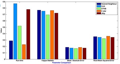
a) No feature selection

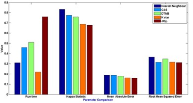
b) NBBBAT feature selection

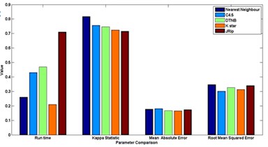
c) PNNBBAT feature selection

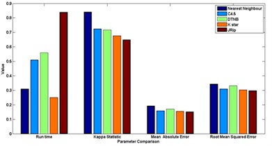
d) OPFBBAT feature selection

Table 7Simulation errors of the classifiers

Feature selection algorithm	Scheme title	Classification algorithm	Mean abs. error	Root mean squared error	Relative abs. error (%)	Root relative squared error (%)
No feature selection	Scheme-1	Nearest neighbour	0.1868	0.3536	35.6514	72.3389
	Scheme-2	C4.5	0.1765	0.3436	34.5753	67.2316
	Scheme-3	DTNB	0.1692	0.3234	34.1040	72.5488
	Scheme-4	K star	0.1851	0.3603	36.3088	76.9163
	Scheme-5	JRip	0.1763	0.3432	33.5350	77.0213
NBBBAT	Scheme-6	Nearest neighbour	0.1898	0.3655	36.2561	67.4199
	Scheme-7	C4.5	0.1871	0.3142	35.7119	62.6599
	Scheme-8	DTNB	0.1788	0.3481	35.0389	73.2075
	Scheme-9	K star	0.1623	0.3159	32.7132	71.6860
	Scheme-10	JRip	0.1597	0.3109	31.1891	74.5798
PNNBBAT	Scheme-11	Nearest neighbour	0.1783	0.3471	35.9381	78.8812
	Scheme-12	C4.5	0.1803	0.3010	36.3413	73.3120
	Scheme-13	DTNB	0.1678	0.3267	33.3218	75.6528
	Scheme-14	K star	0.1659	0.3130	33.4388	73.8726
	Scheme-15	JRip	0.1745	0.3397	35.1722	77.2584
OPFBBAT	Scheme-16	Nearest neighbour	0.1923	0.3444	38.7600	71.7819
	Scheme-17	C4.5	0.1592	0.3099	32.0884	66.7139
	Scheme-18	DTNB	0.1708	0.3325	34.4264	68.8440
	Scheme-19	K star	0.1556	0.3029	31.3627	77.2241
	Scheme-20	JRip	0.1527	0.2973	30.7782	70.3052

In general [31] considers 0-0.20 as slight, 0.21-0.40 as fair, 0.41-0.60 as moderate, 0.61-0.80 as substantial, and 0.81-1 as almost perfect. Kappa > 0.75 as excellent, 0.40-0.75 as fair to good, and < 0.40 as poor. In this present work the Kappa score for the selected algorithms is around 0.62-0.72. Based on the Kappa Statistic criteria, the accuracy of this classification purposes is substantial. Nearest neighbour classifier gives good status of 0.84 Kappa value and lead the list of results.

The simulation error rate of the classification process are listed in the Table 6. In this experimental analysis a very commonly used indicators such as mean of absolute errors and relative absolute errors that belong to regression absolute measure were implied. Relative absolute error is derived from the regression absolute measure component, similarly root mean square error is derived from regression mean measure component. An algorithm which has a lower error rate will be preferred as it has more powerful classification capability and ability in terms of machine learning fields.It is discovered that the lowest error is found in JRip classifier in the whole group of scheme in most of the cases.

7. Conclusions

This paper presents a new approach for diagnosing the faults in gears using EEMD, HBBA and standarded classification algorithms. EEMD is used to extract characteristics from the non-stationary signal. Statistical feature vectors arrived from IMFs of EEMD on both time and frequency domain vibration signals of various faultless and faulty conditions of a gearbox were used in this methodology. Meanwhile, in order to remove the redundant and irrelevant information features swarm intelligence algorithm, HBBA is implemented and the algorithm showed promising results in optimized feature selection process as well in prediction results.To compare the success rates, the different schemes based on hybrid binary bat algorithm (HBBA) along with and classification metrics such as Nearest neighbours, C4.5, DTNB, K star and JRip are performed without feature selection and after feature selection process. The final comparison results indicate the effect of feature extraction based on EEMD and feature selection based on the HBBA techniques. All together, EEMD IMFs extracted features optimized by optimal path forest embedded with binary bat algorithm and nearest neighbour scheme give a better result based on classification accuracy, and in contrast, Jrip also gives a better results with respect to error catagory compared to other schemes in the same condition in gear fault diagnosis.

References

McFadden P. D. Detection fatigue cracks in gears by amplitude and phase demodulation of meshing vibration. Journal of Vibration and Acoustics, Vol. 108, Issue 4, 1986, p. 165-170.

Search CrossRef
Antoni J., RandallR. B. Differential diagnosis of gear and bearing faults. Journal of Vibration and Acoustics, Vol. 124, Issue 2, 2002, p. 165-171.

Search CrossRef
Dalpiaz G., Rivola A., Rubini R. Effectiveness and sensitivity of vibration processing techniques for local fault detection in gears. Mechanical Systems and Signal Processing, Vol. 4, 2000, p. 387-412.

Search CrossRef
De Almeida R. G. T., Da Silva Vicente S. A., Padovese L. R. New technique for evaluation of global vibration levels in rolling bearings. Shock and Vibration, Vol. 9, 2002, p. 225-234.

Search CrossRef
Andrade F. A., Esat I., Badi M. N. M. Gearbox fault detection using statistical methods, time-frequency methods (STFT and Wigner-Ville distribution) and harmonic wavelet – A comparative study. Proceedings of the COMADEM’99, Chipping Norton, 1999, p. 77-85.

Search CrossRef
Meng Q., Qu L. Rotating machinery fault diagnosis using Wigner distribution. Mechanical Systems and Signal Processing, Vol. 5, 1991, p. 155-166.

Search CrossRef
Staszewski W. J., Tomlinson G. R. Application of the wavelet transform to fault detection in a spur gear. Mechanical Systems and Signal Processing, Vol. 8, 1994, p. 289-307.

Search CrossRef
Rubini R., Meneghetti U. Application of the envelope and wavelet transform analyses for the diagnosis of incipient faults in ball bearings. Mechanical Systems and Signal Processing, Vol. 15, 2001, p. 287-302.

Search CrossRef
Aretakis N., Mathioudakis K. Wavelet analysis for gas turbine fault diagnostics. Journal of Engineering for Gas Turbines and Power, Vol. 119, 1997, p. 870-876.

Search CrossRef
Lei Y., He Z., Zi Y. Application of the EEMD method to rotor fault diagnosis of rotating machinery. Mechanical Systems and Signal Processing, Vol. 23, 2009, p. 1327-1338.

Search CrossRef
Lee S. Acoustic diagnosis of a pump by using neural network. Journal of Mechanical Science and Technology, Vol. 20, Issue 12, 2006, p. 2079-2086.

Search CrossRef
Yang B. S., Han T., Hwang W. W. Fault diagnosis of rotating machinery based on multi-class support vector machines. Journal of Mechanical Science and Technology, Vol. 19, Issue 3, 2005, p. 846-859.

Search CrossRef
Lei Y., Zuo M. J. Gear crack level identification based on weighted k nearest neighbor classification algorithm. Mechanical Systems and Signal Processing, Vol. 23, Issue 5, 2009, p. 1535-1547.

Search CrossRef
Bin G. F., Gao J. J., Li X. J. Early fault diagnosis of rotating machinery based on wavelet packets – empirical mode decomposition feature extraction and neural network. Mechanical Systems and Signal Processing, Vol. 27, 2012, p. 696-711.

Search CrossRef
Bartelmus W., Zimroz R. Vibration condition monitoring of planetary gearbox under varying external load. Mechanical Systems and Signal Processing, Vol. 23, Issue 1, 2009, p. 246-257.

Search CrossRef
Ibrahim G., Albarbar A. Comparison between Wigner-Ville distribution and empirical mode decomposition vibration-based techniques for helical gear box monitoring. Proceedings of the Institution of Mechanical Engineers, Part C: Journal of Mechanical Engineering Science, Vol. 225, 2011, p. 1833-1846.

Search CrossRef
Žvokelj M., Zupan S., Prebil I. Non-linear multi variate and multi scale monitoring and signal denoising strategy using kernel principal component analysis combined with ensemble empirical mode decomposition method. Mechanical Systems and Signal Processing, Vol. 25, 2011, p. 2631-2653.

Search CrossRef
Huang N. E., Shen Z., Long S. R., Wu M. C., Shih H. H., Zheng Q., Yen N. C., Tung C. C., Liu H. H. The empirical mode decomposition and the Hilbert spectrum for nonlinear and non-stationary time series analysis. Proceedings of the Royal Society of London. Series A: Mathematical, Physical and Engineering Sciences, Vol. 454, 1998, p. 903-995.

Search CrossRef
Wu Z., Huang N. E. Ensemble empirical mode decomposition: a noise-assisted data analysis method. Advances in Adaptive Data Analysis, Vol. 1, 2009, p. 1-41.

Search CrossRef
Lei Y. G., He Z. J., Zi Y. Y., Hu Q. Fault diagnosis of rotating machinery based on multiple ANFIS combination with gas. Mechanical Systems and Signal Processing, Vol. 21, Issue 5, 2007, p. 2280-2294.

Search CrossRef
Yang X. Bat algorithm for multi-objective optimization. International Journal of Bio-Inspired Computation, Vol. 3, Issue 5, 2011, p. 267-274.

Search CrossRef
Papa J. P., Falcao A. X., Suzuki C. T. N. Supervised pattern classification based on optimum-path forest. International Journal of Imaging Systems and Technology, Vol. 19, Issue 2, 2009, p. 120-131.

Search CrossRef
Webb G. I. Naive Bayes. Encyclopedia of Machine Learning. Springer, New York, NY, USA, 2010, p. 713-714.

Search CrossRef
Yu S. N., Chen Y. H. Electrocardiogram beat classification based on wavelet transformation and probabilistic neural network. Pattern Recognition Letters, Vol. 28, Issue 10, 2007, p. 1142-1150.

Search CrossRef
Darrell T., Indyk P., Shakhnarovich G. Nearest Neighbor Methods in Learning and Vision: Theory and Practice. MIT Press, 2006.

Search CrossRef
Quinlan Ross C4.5: Programs for Machine Learning. Morgan Kaufmann Publishers, San Mateo, CA, 1993.

Search CrossRef
Hall Mark, Frank Eibe Combining naive bayes and decision tables. Proceedings of the 21st Florida Artificial Intelligence Society Conference (FLAIRS), 2008, p. 318-319.

Search CrossRef
Cleary John G., Trigg Leonard E. K*: an instance-based learner using an entropic distance measure. 12th International Conference on Machine Learning, 1995, p. 108-114.

Search CrossRef
Cohen William W. Fast effective rule induction. 12th International Conference on Machine Learning, 1995, p. 115-123.

Search CrossRef
WEKA, http://www.cs.waikato.ac.nz/~ml/weka.

Search CrossRef
Fleiss J. L., Cohen J. The equivalence of weighted kappa and the intra class correlation coefficient as measures of reliability. Educational and Psychological Measurement, Vol. 33, 1973, p. 613-619.

Search CrossRef

About this article

Received

20 December 2014

Accepted

10 March 2015

Published

15 May 2015

SUBJECTS

Fault diagnosis based on vibration signal analysis

Keywords

test rig

fault diagnosis

ensemble empirical mode decomposition

hybrid binary bat algorithm

machine learning classification algorithms

This is an open access article distributed under the Creative Commons Attribution License, which permits unrestricted use, distribution, and reproduction in any medium, provided the original work is properly cited.