Abstract
This paper proposes a new rolling bearing fault diagnosis method based on adaptive multiscale fuzzy entropy (AMFE) and support vector machine (SVM). Unlike existing multiscale Fuzzy entropy (MFE) algorithms, the scales of AMFE method are adaptively determined by using the robust Hermite-local mean decomposition (HLMD) method. AMFE method can be achieved by calculating the Fuzzy Entropy (FuzzyEn) of residual sums of the product functions (PFs) through consecutive removal of high-frequency components. Subsequently, the obtained fault features are fed into the multi-fault classifier SVM to automatically fulfill the fault patterns recognition. The experimental results show that the proposed method outperforms the traditional MFE method for the nonlinear and non-stationary signal analysis, which can be applied to recognize the different categories of rolling bearings.
1. Introduction
The rolling bearings are widely used and crucial components in rotating machinery and their condition monitoring techniques are always a central topic for the maintenance of rotating machinery [1]. Because of the direct relationship between the vibration and the structure of the rotating machine, numerous researches have been focused on the vibration analysis method in recent years [2, 3]. In general, vibration analysis method can be summarized into three steps: data acquisition, fault feature extraction and fault pattern classification. Due to the nonlinear and non-stationary characteristics of the machine fault vibration signals, it is difficult to complete the recognition of the machine working conditions only in the time or frequency domain. How to obtain fault feature information from the vibration signals has become a crux in the fault diagnosis.
Recently, several nonlinear parameter estimation techniques have been developed to extract fault features from the measured signals. Pincus put forward a statistical measure method, named approximate entropy (ApEn), which was successfully applied to physiological time series analysis [4]. Nevertheless, ApEn algorithm counts each sequence as matching itself, which would introduce a bias. To avoid the disadvantage of ApEn, Richman and Moorman proposed a modified version of ApEn, called Sample entropy (SampEn) [5]. Although SampEn can improve performance, it results in an unacceptable result when applied to actual data analysis. Recently, an improved approach of SamEn, fuzzy entropy (FuzzyEn) was proposed by Chen [6], which replaced the Heaviside function with fuzzy membership function, which has a better continuity. However, all the above methods are defined to quantify the irregularity and self-similarity of signal in a single scale, which may lead to misleading results in real time series analysis. In regard to this disadvantage, Costa [7] put forward coarse-grained procedure to estimate the complexity of the original signal over a range of scales, known as Multiscale Entropy (MSE). Multi-scale entropy (MSE) was validated by applying to rolling bearing fault diagnosis by Wu et al. [8]. In order to enhance the evaluating accuracy, the concept of the coarse-graining procedure combined with FuzzyEn (MFE) was developed to measure the self-similarity of original data by Zheng et al. [9]. Unfortunately, the coarse-grained procedure in MFE is essentially a linear smoothing and decimation of the signal [IEEEtrans]. As a result, the MFE algorithm can’t reflect the presence of dominant local trends. What's more, linear operations of coarse-grained procedure is not well adapted to nonlinear and non-stationary actually measured vibration signals [10, 11]. There remains a need for a reliable method that can overcome the weakness of MFE.
In this pape, a new approach called adaptive mutiscale fuzzy entropy (AMFE) is proposed to calculate fuzzy entropy over multiple adaptive scales, which are determined by the Hermite-local mean decomposition (HLMD). LMD is a novel adaptive time-frequency analysis method, which can adaptively decompose any multi-component signal into a number of product functions (PFs) and a residual [12]. The PFs essentially represent locality in time and oscillatory mode (scale) of the original signal. As a novel time-frequency analysis algorithm, some technical difficulties are encountered in the practical application of LMD method [13]. In original LMD algorithm, moving average (MA) approach is performed to construct the local mean function and envelope estimate function in the sifting process, it is time-consuming and may result in inaccurate decomposition results. To solve the problem, Ma Z. Q. introduced the cubic spline interpolation approach to construct the local mean function and envelope estimation function called Spline-LMD (SLMD) [14]. However, we find that the SLMD often generate the series distortion phenomena. Hence, Hermite-LMD (HLMD) method is proposed in this paper, which uses Hermite interpolation to construct the local mean function and envelope function. By virtue of good shape preserving characteristics of Hermite interpolation, the smoothing errors of MA are decreased, leading to a significant performance enhancement.
Based on the advantages of HLMD, AMFE method can be achieved by calculating the Fuzzy Entropy (FuzzyEn) of residual sums of the PFs (scales) through consecutive removal of high-frequency components. Since the scales in AMFE is determined by the time series data, which should be more suitable to characterize the underlying nonlinear dynamics and complexity of the time series data. Therefore, AMFE is applied to extract the fault features from the vibration signals in this paper.
Naturally, after the fault features extraction with AMFE, a multi-fault classifier is employed to automatically identify the fault patterns. Support vector machine (SVM) based on statistical learning theory was put forward by Vapnik, SVM had been demonstrated to be more effective in making a reliable decision for a smaller number of datasets compared with artificial neural networks (ANN) [15]. Since SVM has high accuracy and good generalization capabilities, it has been widely applied in fault diagnosis and classification field [16].
This paper is organized into five sections. In Section 2, the main steps of HLMD are introduced and the comparisons of simulation signal analysis among LMD, HLMD and SLMD are discussed, which show that the better performance can be obtained by using HLMD method. Section 3 describes the basis of AMFE and validates the superiority of AMFE using the simulation signal. Section 4 illustrates the proposed fault diagnosis method based on AMFE and SVM and discusses experimental results. Finally, conclusions are drawn in Section 5.
2. HLMD algorithm
2.1. HLMD method and calculation procedures
In LMD method, a multi-component signal can be decomposed into a sum of PF components, each of which is the product of an envelope signal and a pure FM signal. Compared with EMD method, the prominent advantage of LMD is that it directly gives access to the calculations of the IA and IF of each PF, avoiding performing the Hilbert transform (HT). However, the original LMD method employs the moving algorithm (MA) approach to compute the local mean function and envelope estimation function , which can be easily affected by noise of the inspected signals and produce errors in the smoothing process [13]. Also the sliding step sizes selection is an unsolved problem in the MA algorithm.
To overcome the drawbacks of original LMD, Deng L. introduced the cubic spline interpolation approach to construct the local mean function and envelope estimation function [16]. However, the envelopes constructed by cubic spline interpolation may produce outstanding over and undershoot problems [17]. In this paper, the cubic Hermite interpolation approach is introduced to obtain local meanand envelope estimation functions.
The definition of the cubic Hermite interpolation is given as follows.
Given a series of discrete date and , the is the value at time ( 0, 1, 2,…, ), is the first derivative at each time , , and is any real numbers. Then in each can be written as:
where , , and are basis functions of the cubic Hermite interpolation, which can be expressed as:
Based on the computation of local mean function and envelope estimation function using cubic Hermite interpolation. For a given signal , the calculation steps of HLMD method can be summarized as follows:
Step 1: Identify all local extrema of the original signal , and the mirror-symmetric extension method is used to extend endpoints to obtain a new extreme point sequence .
Step 2: Calculate the upper envelop and lower envelop of the signal being analyzed by using cubic Hermite interpolation algorithms.
Step 3: Compute local mean function and envelope estimation function using the upper and lower envelopes according to Eq. (3) and Eq. (4):
Step 4: The local mean function is subtracted from the original data :
where is then amplitude demodulated by been divided by:
The envelope of can then be calculated by step (1) and (2). If the envelope function 1, stop the procedure and take as the first purely frequency modulated signal. If the envelope function 1, regard as the original singal and repeate the steps (1)-(4) continues times until a purely frequency modulated signal is obtained:
in which:
The objective of the itearation is to obtain a signal whose envelope function should satisfy 1.
Step 5: The corresponding envelope is obtained by Eq. (9):
The envelope function is then multipied by the purely frequency modulated signal and then the first product function can be written as:
In fact, the instantaneous amplitude of is and the instantaneous frequency of can be calculated by the pure frequency modulated signal according to Eq. (11):
Step 6: This derived is then subtracted from the original time series , resulting in a new function , which represents a smoothed version of the original data since the highest frequency oscillations have been removed from it. Regard as a new data and repeat the above procedure times until is a constant or contains no more oscillations:
Thus, the original signal can be reconstructed product functions and a residual according to:
where is the residue and is the number of PF components .
It should be noted that is envelope estimation function, and denotes the th component in the th iterations. In practice, a variation can be determined in advance. If , then iterative process would be stopped. Also, the decomposition stops when the becomes monotonic function, usually, the monotonic criterion is determined by the number of the extrema of . If the number of the extrema of is no more than 3, then the is monotonic and the decomposition is completed.
2.2. Application to simulation signals
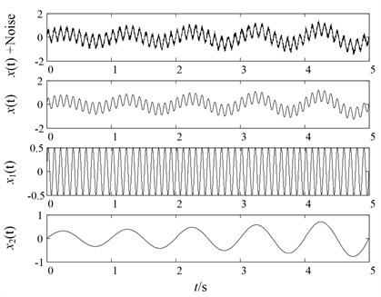
In order to validate the effectiveness of the proposed HLMD method, a simulation signal is employed to conduct the comparisons among original LMD, HLMD and SLMD. The simulation signal consists of an AM-FM signal , an AM signal and a white noise, set sampling frequency 1000 Hz, the sampling time is 5 seconds:
The waveforms of simulation signals are shown in Fig. 1.
Fig. 1Simulation signal and its three components
To begin with, original LMD, HLMD and SLMD methods are all applied to decompose the noisy signal in Eq. (14). The decomposition results of the three methods are represented in Fig. 2, Fig. 3 and Fig. 4, respectively. It should be noted that the boundary conditions of the simulation signal have been handled by the mirror-symmetric extension [18] and the iteration stop condition is , where 10-4.
Fig. 2Original LMD decomposition results of noisy signal
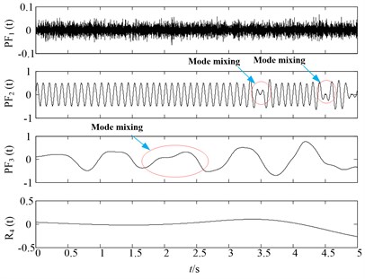
Fig. 3HLMD decomposition results of noisy signal
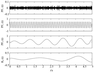
It can be observed from Fig. 2 that the first PF component of original LMD method is the noisy signal and second and third are corresponding to the , of the simulation signal. However, it can be easily found that the slight distortion phenomena occur in the second and third components of original LMD. While in the Fig. 3, there are no such distortion phenomenon in the and of HLMD, resulting in more accurate decomposition results. For comparison purpose, the SLMD is also employed to decompose the noisy signal. Fig. 4 shows the decomposition results of SLMD method, from which we can find that SLMD decomposition results are serious distorted, losing the physical meaning.
Fig. 4SLMD decomposition results of noisy signal
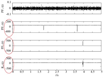
Secondly, to further compare the decomposition ability of original LMD, HLMD and SLMD methods, the demodulation technique is utilized to calculate instantaneous frequency (IF) and instantaneous amplitudes (IA) and the time-frequency representation (TFR) of the PFs obtained by the three methods are shown in Fig. 5. From Fig. 5(a) (the TFR of PFs obtained by the original LMD method), it is clear that the distortion appears in the second and third PF of original EMD (with IF 10 Hz and 2 Hz, respectively), which is due to the errors in the smoothing process using the MA. Conversely, the TFR of PFs derived from HLMD can ameliorate the fluctuation phenomenon with less distortion. Furthermore, the first horizontal line in Fig. 5(b) (with IF 10 Hz) has a narrower bandwidth than that of original LMD method. Additionally, it can be easily observed that the TFR of PFs derived from SLMD in Fig. 5(c) are totally anamorphic. Therefore, the above analysis results verify that HLMD can significantly restrict the mode mixing phenomena and get more accurate IF and IA compared with other two methods.
Fig. 5The time-frequency distribution of the PFs derived from the three LMD methods: a) the time-frequency distribution of original LMF method, b) the time-frequency distribution of HLMD method and c) the time-frequency distribution of SLMD method
a)
b)
c)
Lastly, three assessing indexes are chosen to assess the decomposition performance. Orthogonal index (), root mean squared error (RMSE) and calculation efficiency are considered as assessing indicators. Firstly, the definitions of the three assessing indicators are describes as follows. The is defined as [19]:
where is the number of PFs. is the length of the . and are the th and th PF at sifting step , respectively. is the original signal and is the residual after LMD decomposition. Theoretically, the PFs and the final residual obtained by LMD decomposition are expected to be mutually orthogonal, which means the index is proposed to be zero. Therefore, the smaller (more close to zero) means the better decomposition results. Secondly, the RMSE definition is as follows:
where and are the original defined component and the corresponding decomposed component, respectively. RMSE is utilized to assess the decomposition accuracy. In theory, the RMSE value should be zero, hence, the smaller RMSE value indicates that the obtained mono-components are more precise and more close to real and in Eq. (14). Eventually, we need to discuss the calculation efficiency of the three methods. The computer with 3.3 GHz i3-Core CPU, 4.0 GB RAM and MATLAB (R2010b) platform are employed to conduct the simulation.
Since the decomposition results of SLMD are serious distortion, it has been omitted in the following comparisons. We only conduct the comparisons between original LMD and HLMD methods, the compassion results are shown in Table 1.
Table 1Three assessing indicators comparison for the original LMD and HLMD methods
Methods | Consuming time (s) | Orthogonal index | ||
RMSE | RMSE | |||
Original LMD method | 0.1852 | 0.2393 | 125.72 | 0.0120 |
HLMD method | 0.0578 | 0.0756 | 2.78 | 0.0014 |
We can draw the following conclusions from Table 1. Firstly, it can be found that the RMSE values of , (corresponding to the and of original signal) derived from HLMD method (0.0578, 0.0756) are smaller than that of original LMD method (0.1852, 0.2393), it indicate that the decomposition results of HLMD are more close to the real mono-component of the original signal and , respectively. Secondly, the consuming time of original LMD is 125.72 s, which is much more than that of HLMD method. Lastly, compared with original LMD method, HLMD has a smaller value, which shows that HLMD method is super to original HLMD method in the orthogonality.
The comparative results illustrate that HLMD consumes less computation time and generates more accurate decomposition results than original LMD. The above analysis results can be explained in the following way.
Since the cubic Hermite approach is first-order smoothness, it not only has enough flexibility to fit the local extreme points of the signal but also has an excellent conformal characteristic, which is more suitable for fitting envelope of the rolling bearing vibration signal than the cubic Hermite approach.
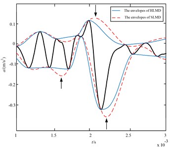
Furthermore, a section of data intercepted from the simulation signal in the sifting process is taken to find out the cause for the above comparison results, which is shown in Fig. 6. It is easy to find that envelope-lines fitted by the cubic spline interpolation in red dashed line have serious over and undershoot problems, which are denoted by arrows in Fig. 6. Whereas, the envelope-lines fitted by Hermite interpolation in blue line can eliminate the over and undershoot problems of cubic spline interpolation obviously. Hence, the HLMD can obtain more reliable envelope-lines and accurate decomposition results.
To summarise, the original LMD method uses MA to calculate the local mean function and envelope estimate function , which can be easily affected by noise of the inspected signals and generate errors in the smoothing process [13, 14]. Whereas, HLMD adopts the cubic Hermite interpolation method instead of MA to construct the local mean function and envelope estimate function . The cubic Hermite interpolation has a continuous first derivative property at the node and the obtained lines have an excellent conformal characteristic, which can decrease smoothing errors of MA effectively. Therefore, in this paper HLMD method is taken to preprocess the vibration signals, resulting in a series of scale-dependent PFs.
Fig. 6The envelopes of the Hermite interpolation (blue line) and optimized rational spline (red dashed line) interpolation
3. Adaptive multi-scale fuzzy entropy (AMFE)
3.1. The basis of multi-scale fuzzy entropy (MFE) and the disadvantages
The definition and calculation procedures of sample entropy (SE) are described by [20]. Since the similarity definition of the two vectors is mainly according to the Heaviside function, which is jumping and not according with the boundaries of the actual times series, whereby the two classes are mostly ambiguous. To overcome the disadvantages of SE, fuzzy entropy (FE) is developed, which used the Gaussian function to replace the Heaviside function. The detailed steps of FuzzyEn are given in literature [6]. Recently, the multi-scale analysis algorithm was developed by Costa [7] to quantify the complexity of time series in different scales. Based on the concept of multi-scale analysis, MFE method was proposed by Zheng et al. [9], which can measure the complexity of time series over the different scales.
MFE algorithm contains two steps. Firstly, apply the coarse-grained procedure to get multiple scale time series from the original time series. Then, calculate the FuzzyEn at each coarse-grained time series. Two procedures of MFE algorithm are briefly described as follows.
1) To obtain the coarse-grained time series at a scale factor of , the original time series is divided into disjointed windows of length τ, and the data points are averaged inside each window. Namely, the coarse-grained time series at a scale factor of ( is a positive integer), can be constructed according to Eq. (17):
2) In MFE analysis, the FuzzyEn of each coarse-grained time series is calculated based on FuzzyEn calculation steps and then plotted as the function of the scale factor , which can be expressed as:
Note that the in the calculation for different scales is same, which is obtained by the . is the standard deviation of the original time series.
However, in the MFE method, the scales are determined by the “coarse-grained” procedure. From Eq. (17), it can be found that the length of the coarse grained time series is equal to the length of original time series divided by the scale factor . Namely, the coarse-grained procedure of MFE is essentially a linear smoothing and decimation of the original time series, eliminating high-frequency components. Due to the linear operations of coarse-grained procedure, it is unsuitable to extract the fault feature using MFE in the different scales when analyzing the nonlinear and non-stationary signals.
3.2. AMFE algorithm
To overcome the disadvantages of MFE, a novel fault feature extractor called adaptive multiscale entropy (AME) is proposed in this paper. AMFE can estimate the entropy of the signal over multiple adaptive scales that are intrinsically determined using HLMD method. The AMFE is mainly composed of three procedures: (1) Perform HLMD method to decompose the rolling bearing data into a sum of PFs under different scales; (2) Generate the adaptive scales by consecutively removing the PF component with high frequency; (3) Calculate the FuzzyEn of the obtained adaptive scales. Namely, the consecutively removing PF component procedures essentially represent the mutiscale low-pass filtering of the original signal. The main steps of AMFE are described as follows.
Algorithm: Adaptive mutiscale fuzzy entropy (AMFE):
1) The measured rolling bearing vibration signals are firstly decomposed by HLMD to acquire a set of components in different scales and the residual is considered as the last component, denoted as , ,…, :
2) Generate the adaptive scales by consecutively removing the component with high frequency from the original signal via Eq. (20):
where denotes the number of the components.
3) Calcluate the FuzzyEn value of the obtaied adaptive scales to fulfill the AMFE values:
here set the 0.15, 2 and 2.
From the above steps of AMFE, we can find that the procedures of obtaining different scales in AMFE are really like the “coarse-grained” procedure. However, the scales in AMFE are obtained using HLMD, which are adaptive to the time series. Meanwhile, since the HLMD is complete data-driven time-frequency technique, the fault information stored in different frequency components are preserved, allowing an efficient search of discriminating features.
3.3. Comparison between AMFE and MFE
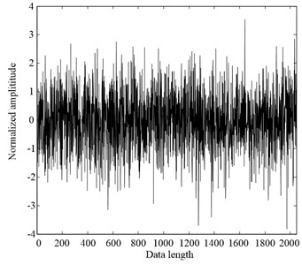
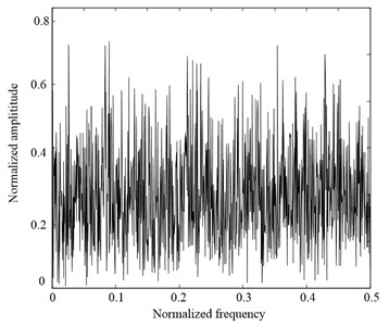
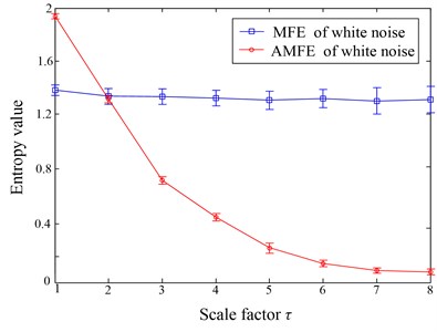
In order to investigate the estimate performance of AMFE method, a white noise simulation signal is utilized to conduct the comparisons between AMFE and MFE methods. The waveforms of the white noise and its Fourier transform spectrum are illustrated in Fig. 7. As can be seen from its spectrum, the complexity of white noise is uniform distribution.
AMFE and MFE methods are both used to analyze 100 independent white noises, each of which contains 1000 data points. The error bar calculated from 100 independent noise signals at each scale are shown in Fig. 8. The following conclusions can be drawn from Fig. 8. Firstly, the FuzzyEn curve of white noise obtained by AMFE method decreases monotonically with scale increasing, which is consistent with the conclusions drawn in literature [21]. In contrast, the FuzzyEn curve obtained by traditional MFE method is nearly independent of scale, which can’t reflex the dynamic change of time series. It is well known that the error bar at each scale indicates the standard deviation (SD) of a FuzzyEn value. As seen the error bar of white noise in Fig. 8, the SD of AMFE is less than that of MFE, which indicate that AMFE has a more stable performance in estimating the complexity of the time series.
Fig. 7The waveform and FT spectrum of white noise
a)
b)
Fig. 8AMFE and MFE analysis of white noise
4. The proposed fault diagnosis method and experimental signal analysis
4.1. The fault feature extraction based on AMFE and SVM
Based on the superiorities of AMFE and SVM, a novel rolling bearing fault diagnosis approach is presented in this paper, it can be summarized as follows:
1) When the machine operates under different working conditions, the vibration signals are measured by acceleration sensors at a sampling frequency . The sensor-based vibration signals are preprocessed by the HLMD method and a series of PF components are obtained. Remove consecutively the PF component with high frequency from the original signal to acquire the adaptive scales , denoted as fine-course procedure;
2) FuzzyEn algorithm is employed to calculate the obtained adaptive scales (t). In the whole paper, we define the number of adaptive scales from 1 to 6 ( 1 to 6) and the FuzzyEn values of each coarse grained time series obtained by Eq. (20) is computed with the dimension 2 and tolerance 0.15.
3) The obtained fault features are fed into fault classifier SVM to identify the different health conditions.
4.2. Experimental validation
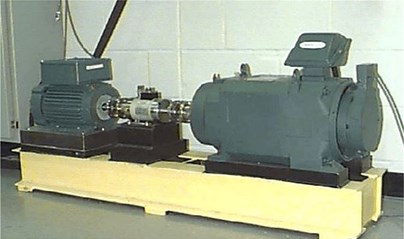
In this section, an actual rolling bearing data is utilized to examine the utility of proposed algorithm. The test bearing data was obtained from the Bearing Data Center of Case Western Reserve University Bearing Data Center [22]. Fig. 9 gives the platform of the experiment system. The 6205-2RS JEM SKF deep groove ball bearing is used in this test. The vibration signals of bearing were collected under four conditions including normal condition, the ball fault condition, the outer race fault condition and the inner race fault condition. In each bearing fault condition, the bearing was seeded with signal point using the electro-discharge machining with fault diameters of 0.1778 mm, 0.3556 mm, 0.5334 mm and 0.7112 mm. An accelerometer was mounted on the front section end to collect the vibration signal. In addition, the sampling frequency is 12000 Hz and the shaft rotating speed of the motor is 1797 rpm without motor load.
Fig. 9The platform of rolling bearing experiment system
To demonstrate the effectiveness of the methodology can be applied to recognize the different categories and severities of rolling bearings. The experimental vibration signals are composed of four fault categories and each fault category contains different levels of severity. Based on the different fault categories and various fault degrees, actually, the experimental analysis is an seven-class recognition problem. The vibration signals in the experiment are divided into several non-overlapping segments with the length of 2,000. There are 40 samples for each bearing condition, and there are total 280 samples, in which 140 samples will be randomly selected as the training data, and the residual 140 samples will be testing data. The detailed numbers of samples description for each bearing condition are shown in Table 2.
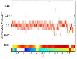
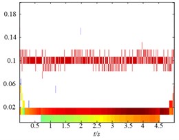
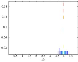
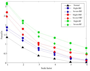
Fig. 10 gives the time domain waveforms of vibration signals under four fault categories case, respectively. According to procedures in Section 4.1, HLMD method is firstly adopted to decompose the vibration signal into a sum of mono-components, the decomposition results of bearing at normal condition is shown in Figs. 11 (other bearing working conditions are omitted for saving space). Subsequently, the AMFE is completed by calculating the FuzzyEn of residual sums of the PFs though consecutively removing the PF component with high frequency from the original signal. The obtained results of AMFE is shown in Fig. 12, from which it can be observe that the FuzzyEn exhibits the decreased trend as the fine PFs with high frequency are consecutively removed. Moreover, the four health conditions can be significantly distinguished using AMFE method.
Table 2The detailed description of the experimental data sets
Fault class | Fault diameter (mm) | Fault severity | Number of training data | Number of test data | Class label |
IRF | 0.1778 | Slight | 20 | 20 | 1 |
0.5334 | Severe | 20 | 20 | 3 | |
ORF | 0.1778 | Slight | 20 | 20 | 4 |
0.5334 | Severe | 20 | 20 | 5 | |
BF | 0.1778 | Slight | 20 | 20 | 6 |
0.5334 | Severe | 20 | 20 | 7 | |
Normal | 0 | 20 | 20 | 8 |
Fig. 10The vibration signals of each rolling bearing condition
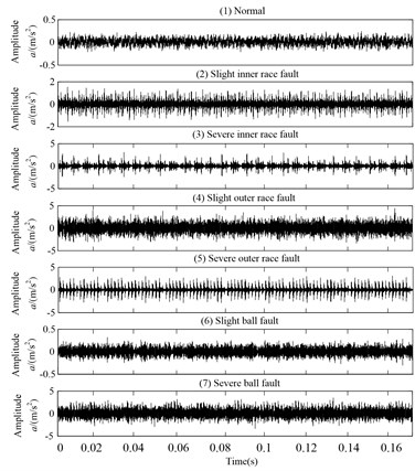
Fig. 11HLMD decomposition results of bearing with normal condition
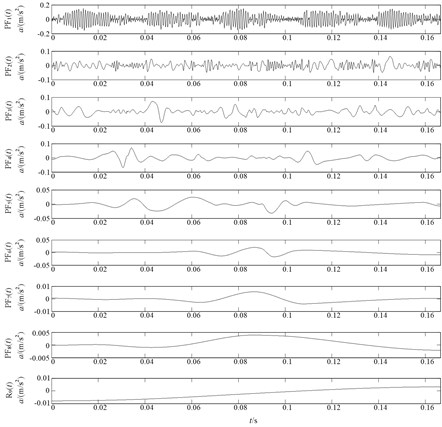
Fig. 12AMFE over 6 scales of the original vibration signal
Naturally, according to the flowchart of AMFE and SVM algorithm, the obtained fault features are fed into fault classifier SVM to identify the different health conditions. As mentioned above, 140 groups of data are selected randomly as training set to train the SVM-classifier and the remaining 140 group of data are taken as testing set to test the trained SVM-classifier. In addition, PSO algorithm is applied to calculate the optimal penalty parameter and kernel parameter according to the training data [23]. Hence the testing set are fed into the trained model to achieve the fault identification, and the output testing results are shown in Table 3. It can be found no samples of the four fault types are misclassified, and the training and testing accuracy are both 100 %, which demonstrate the proposed AMFE and SVM method is feasible and effective in the rolling bearing fault diagnosis.
Table 3The classification results of the SVM-classifier using AMFE
Fault class | Class label | Number of training samples | The number of misclassified samples | Number of testing samples | The number of misclassified samples | Training accuracies/testing accuracies (%) |
Normal | 1 | 20 | 0 | 20 | 0 | 100/100 |
Slight-IRF | 2 | 20 | 0 | 20 | 0 | 100/100 |
Severe-IRF | 3 | 20 | 0 | 20 | 0 | 100/100 |
Slight-ORF | 4 | 20 | 0 | 20 | 0 | 100/100 |
Severe-ORF | 5 | 20 | 0 | 20 | 0 | 100/100 |
Slight-BF | 6 | 20 | 0 | 20 | 0 | 100/100 |
Severe-BF | 7 | 20 | 0 | 20 | 0 | 100/100 |
In total | 140 | 0 | 140 | 0 | 100/100 |
For comparison purpose, the MFE method is also used to analyze the rolling bearing data, and the fault features obtained by MFE are also fed into SVM for pattern identification. Through the same process in AMFE-SVM method, which includs the number of training and testing samples and the parameter selection of SVM, the classification results based on MFE and SVM are shown in Table 4. It can be easily found that there are one sample with slight and severe inner race fault, severe ball fault as well as three samples with slight ball fault are misclassified, which coincide well with the above analysis. The total testing classification accuracy of 96.4 %, while the corresponding testing classification accuracy of AMFE is 100 %. The comparisons demonstrate that the proposed method can present better distinguishability and superior performance in identifying various fault patterns of rolling bearing.
Table 4The classification results of the SVM-classifier using MFE
Fault class | Class label | Number of training samples | The number of misclassified samples | Number of testing samples | The number of misclassified samples | Training accuracies/testing accuracies (%) |
Normal | 1 | 20 | 0 | 20 | 0 | 100/100 |
Slight-IRF | 2 | 20 | 0 | 20 | 1 | 100/95 |
Severe-IRF | 3 | 20 | 0 | 20 | 1 | 100/95 |
Slight-ORF | 4 | 20 | 0 | 20 | 0 | 100/100 |
Severe-ORF | 5 | 20 | 0 | 20 | 0 | 100/100 |
Slight-BF | 6 | 20 | 0 | 20 | 3 | 100/85 |
Severe-BF | 7 | 20 | 0 | 20 | 1 | 100/100 |
In total | 140 | 0 | 140 | 5 | 100/96.4 |
5. Conclusions
A new fault feature extraction approach called AMFE is proposed to measure complexity of bearing vibration signal in this paper. In the proposed method, HLMD is firstly employed to decompose the vibration signal into a number of scale-dependent PF components. Then the AMFE method is performed by computing the FuzzyEn of the scales obtained by continually subtracting the high-frequency PF components from the signal. For comparison purpose, AMFE method is compared with traditional MFE method by analyzing simulation signal, the comparison results demonstrate AMFE method has a more stable estimation performance than MFE method. Furthermore, the actual rolling bearing fault diagnosis confirms that the proposed methodology can extract more fault information and fulfill the rolling bearing fault diagnosis effectively.
References
-
Abbasion S., Rafsanjani A., Farshidianfar A. Rolling element bearings multi-fault classification based on the wavelet denoising and support vector machine. Mechanical Systems and Signal Processing, Vol. 21, 2007, p. 2933-2945.
-
Feng Z., Zuo M. J. Vibration signal models for fault diagnosis of planetary gearboxes. Journal of Sound and Vibration, Vol. 331, 2012, p. 4919-4939.
-
Zheng J. D., Cheng J. S., Yang Y. A rolling bearing fault diagnosis approach based on LCD and fuzzy entropy. Mechanism and Machine Theory, Vol. 70, 2013, p. 441-453.
-
Pincus S. M. Approximate entropy as a measure of system complexity. Proceedings of the National Academy of Sciences, Vol. 88, 1991, p. 2297-2301.
-
Richman J. S., Moorman J. R. Physiological time-series analysis using approximate entropy and sample entropy. American Journal of Physiology-Heart and Circulatory Physiology, Vol. 278, 2000, p. 2039-2049.
-
Chen W., Zhuang J., Yu W., Wang Z. Measuring complexity using FuzzyEn, ApEn, and SampEn. Medical Engineering and Physics, Vol. 31, 2009, p. 61-68.
-
Costa M., Goldberger A. L., Peng C. K. Multiscale entropy analysis of complex physiologic time series. Physical Review Letters, Vol. 89, 2002, p. 068102.
-
Wu S. D., Wu P. H., Wu C. W. Bearing fault diagnosis based on multiscale permutation entropy and support vector machine. Entropy, Vol. 14, 2012, p. 1343-1356.
-
Zheng J. D., Cheng J. S., Yang Y., Luo S. R. A rolling bearing fault diagnosis method based on multi-scale fuzzy entropy and variable predictive model-based class discrimination. Mechanism and Machine Theory, Vol. 78, 2014, p. 187-200.
-
Amoud H., Snoussi H., Hewson D. Intrinsic mode entropy for nonlinear discriminant analysis. IEEE Signal Processing Letters, Vol. 14, 2007, p. 297-300.
-
Hu M., Liang H. Adaptive multiscale entropy analysis of multivariate neural data. IEEE Transactions on Biomedical Engineering, Vol. 59, 2012, p. 12-15.
-
Smith J. S. The local mean decomposition and its application to EEG perception data. Journal of the Royal Society Interface, Vol. 2, 2005, p. 443-445.
-
Wang Y., He Z., Zi Y. A demodulation method based on improved local mean decomposition and its application in rub-impact fault diagnosis. Measurement Science and Technology, Vol. 20, 2009, p. 02570.
-
Ma Z. Q., Yang W., Kang D. L. Decomposition with LMD of mechanical fault signals based on LabVIEW. Applied Mechanics and Materials, Vol. 278, 2013, p. 1133-1136.
-
Vapnik V. N. The Nature of Statistical Learning Theory. Springerverlag, New York, 1995.
-
Cheong S. M., Oh S. H., Lee S. Y. Support vector machines with binary tree architecture for multi-class classification. Neural Information Processing-Letters and Reviews, Vol. 2, 2004, p. 47-51.
-
Li Y., Xu M., Wei Y., Huang W. An improvement EMD method based on the optimized rational Hermite interpolation approach and its application to gear fault diagnosis. Measurement, Vol. 63, 2015, p. 330-345.
-
Rilling G., Flandrin P., Goncalves P. On empirical mode decomposition and its algorithms. Proceadings of IEEE-EURASIP Workshop on Nonlinear Signal and Image Processing, Grado, Italy, 2003.
-
Zhang K., Cheng J., Yang Y. Product function criterion in local mean decomposition method. Journal of Vibration and Shock, Vol. 30, 2011, p. 84-88.
-
Xiong G. L., Zhang L., Liu H. S., Zou H. J. A comparative study on ApEn, SampEn and their fuzzy counterparts in a multiscale framework for feature extraction. Journal of Zhejiang University Science A, Vol. 11, 2010, p. 270-279.
-
Jiang Y., Peng C. K., Xu Y. S. Hierarchical entropy analysis for biological signals. Journal of Computational and Applied Mathematics, Vol. 236, 2011, p. 728-742.
-
Bearing Data Center. Case Western Reserve University, http://csegroups.case.edu/bearing datacenter/pages/download-data-file.
-
Huang C. L., Dun J. F. A distributed PSO-SVM hybrid system with feature selection and parameter optimization. Applied Soft Computing, Vol. 8, 2008, p. 1381-1391.
About this article
The research is supported by National Natural Science Foundation of China (No. 11172078) and Important National Basic Research Program of China (973 Program-2012CB720003), and the authors are grateful to all the reviewers and the editor for their valuable comments.
