Abstract
Present day requirements for enhanced reliability of rotating machinery have become critical for the manufacturing sector. Every rotating machine exhibits a unique characteristic vibration and acoustic signature. This can be used to identify the defective parts and estimate the present severity of the problem; most importantly, without opening the machine for inspection. Moreover, it aids in the reduction of unscheduled down time, turnaround time and existing noise levels. The paper deals with the vibro-acoustic condition monitoring of metal lathe and development of predictive models for the detection of probable faults using Machine Learning. Experiments were conducted to obtain vibration signatures using accelerometers and the data was further processed while the acoustic signatures were obtained using noise level meters. Results were obtained for idle running, turning and facing operations using a single point cutting tool for constant spindle speeds, feed and depth of cut. The vibro-acoustic signatures of six metal lathe machines were collected over a period of 5 months and the trends obtained were analyzed. The filtered acceleration (g-peak) signatures were compared with the General Machinery Vibration Severity Chart and based on the velocity classification results, the best machine was chosen for the development of predictive models. Vibration as well as acoustic signatures were isolated using filters, empirical relations and manufacturing data. Predictive models were made using machine learning algorithms to predict the failure of the lathe based on its historical data. These models can be used by industries to detect unhealthy trends and identify troublesome parts in the machine which can be then scheduled for maintenance thereby decreasing production downtimes.
1. Introduction
Approximately half of all operating costs in most processing and manufacturing operations can be attributed to maintenance. As a result, machine condition monitoring systems have been gaining considerable importance in the manufacturing industry [1], since they allow for a significant reduction in the machinery maintenance costs, and most importantly, the early detection of potentially disastrous faults. Besides the detection of the early occurrence and seriousness of a fault, it aids in the identification of components that are deteriorating; most importantly, without even opening the machine for inspection.
Machine condition monitoring can be defined as a field of technical activity in which selected physical parameters, associated with machinery operation, are observed for the purpose of determining machine integrity [1-5]. Once this has been estimated, maintenance activities can be scheduled only when needed, which results in optimum use of resources. The main reason for employing machine condition monitoring is to generate accurate, quantitative information on the present condition of a machine, here the lathe, in order to optimally schedule maintenance, achieve maximum productivity, and still avoid unexpected catastrophic failures. It also results in improved risk maintenance and increased machine reliability [2-3]. Vibration monitoring and acoustic emissions [2, 5, 6] are the two most effective and commonly used techniques for condition monitoring of machines.
The paper examines the historical data collected over a period of 5 months to predict the condition of machine using machine learning algorithms [3, 4, 7, 8]. The collected vibration and acoustic data is used with machine learning algorithms to monitor the mechanical condition and derive the approximate time of a functional failure of different parts, resulting in scheduled maintenance. Vibration condition monitoring has been a trusted method for the past thirty years [3-4, 9]. However, the time and effort required to obtain machine signatures is much more as compared to acoustic condition monitoring. The acoustic method has significant advantages in terms of lower costs of experimental setup and the ease of application. The issue of placement of accelerometers and connections to amplifiers is completely eliminated and is instead replaced by a single hassle free acoustic noise level meter.
Condition monitoring analysis has been done in the past for different operations on the Lathe but with a view of detecting failures of the machining tool [10-11]. Here we present two different models to schedule maintenance operations of the lathe machine based on its vibro-acoustic condition monitoring. The approach outlined in this paper is distinct from the previous efforts as it not only predicts the time to failure using acoustic and vibratory levels but also compares the results obtained from the two approaches each, with the help of the two models. Two generic models are developed here and can be used for different lathe machines but with their own specific training data.
2. Condition monitoring process
Data acquisition is the initial and one of the most important phases of Condition Monitoring which involves recording the vibration and acoustic signals of the metal lathe [4, 8]. Signal processing techniques such as Fast Fourier Transform (FFT) are then applied to analyze the data [10, 12]. In order to make the condition monitoring models applicable to the industrial needs, all measurements were taken in a fully functional workshop instead of a closed laboratory environment. This is done to ensure that the models can be used in industries as per requirements. Our proposed model only outlines the methodology to be followed to set up a maintenance scheduling system. However, the general procedure remains the same and can be designed for any machine with its own set of historical training data.
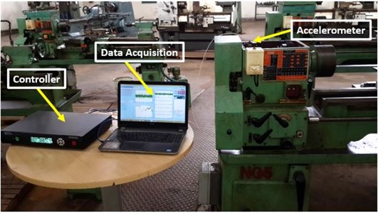
In our scenario, initial set of experiments were carried out on six different metal lathes for three days. In order to obtain vibration signatures, a piezoelectric accelerometer having a sensitivity of 101.3 mV/g is used. After preparing the surface, it is mounted on the bearing housing, perpendicular to the shaft center-line, using adhesives. Alignment of lathe is done prior to mounting. As the output of the accelerometer is of low level and contains some unwanted frequencies, some form of pre-processing is required before analyzing the data. A 4-input, 1-output vibration analyzer system [13] (Spider-81 Vibration Controller System) amplifies the output data of the accelerometer and converts the data into frequency domain using Electronic Data Management (EDM) software. The setup for vibration data acquisition is shown in Fig. 1. The controller shown in the figure consists of the Preamplifier and Spectrum Analyzer.
Fig. 1Vibration data acquisition setup
The acoustic signatures are obtained using a noise level meter [14]. A mesh is designed around the lathe and the measurement point is selected based on the maximum likelihood localization method [15] as shown in Fig. 3. The sound level meter (SLM) is kept at the prescribed safe distance of 20 cm from the base of the lathe machine. The readings are taken in the absence of any external noise field. The setup for acoustic measurements is shown in Figs. 2 and 3 [16].
Fig. 2Acoustic data acquisition setup
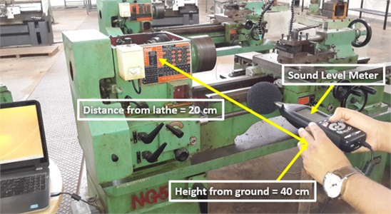
Fig. 3Grid points around lathe machine
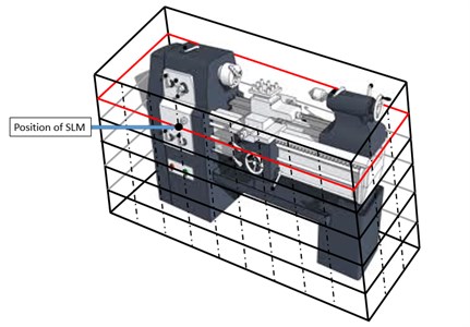
The position of the SLM is indicated in Fig. 3. The red lines denote the plane of vibration of the headstock bearings. All acoustic measurements are taken at this plane’s height which is equal to 40 cm. This height is chosen based on the maximum likelihood principle, according to which the sound intensity at all grid points are not the same and it varies approximately according to the Inverse square law [15, 17] as shown in Eq. (1):
From Eq. (1), it can be inferred that the maximum sound intensity from the headstock bearing would most likely be detected at the point highilighted in Fig. 3. Moreover, the measurements of the peak values at various points on the mesh around the lathe also show the maximum sound intensity at the same point. Hence, we select this point from the mesh to be our measurement point. In the same way, different maximum likelihood points need to be chosen for the development of condition monitoring models of different components of the lathe or different machine parts in industries.
2.1. Status of lathe
To perform the condition monitoring process, we record the vibration and acoustic data of any untested machine until its breakdown which may be due to common industrial failures like fatigue or wear and tear. The vibration and acoustic data obtained at the first breakdown point is used as the threshold value for performing the condition monitoring of similar machines. This might be a slight drawback in case of untested machines as the entire predicitive model can be applied only after the first breakdown. However, this threshold value can also be obtained from manufacturing catalogues or from an identical machine which is due for maintenance. For our experiment, six identical lathe machines were analyzed for vibration specific acceleration values (g-peak) and acoustic peak levels (dB). Considering the g-peak values along with their corresponding frequencies, a comparison was made with the standard Vibration Acceleration General Severity Chart [3]. The g-peak acceleration values obtained for all the six Lathe machines at idle running conditions and at a speed of 1800 rpm is shown in Table 1. The condition of the Lathe so obtained using the Vibration Velocity General Severity Chart [3] is used to classify the lathes into categories – good, fair, smooth and very smooth. This is also shown in Table 1. It is important to note that even though our experiments were done with mild steel as the material, the combination of the Acceleration and Velocity Severity charts is independent of the material being used. However, the classification will vary with the processing speed. But, for the purpose of development and comparison of the vibration and acoustic condition monitoring models, it is necessary to record the training data at a constant processing speed. Hence, Table 1 forms the backbone of the entire process and needs to be formulated for any machine prior to development of the models proposed below.
Table 1Classification of lathes
Lathe machine | Acceleration g-peak | Condition |
Machine A | 0.02041 | Good |
Machine B | 0.01379 | Very smooth |
Machine C | 0.01263 | Very smooth |
Machine D | 0.02458 | Fair |
Machine E | 0.01710 | Smooth |
Machine F | 0.01968 | Smooth |
2.2. Selection of lathe
Machines B and C were observed to be the best machines out of the six lathes as they were the two lathes classified into the very smooth category. This can be seen from the Condition column in Table 1 and the lowest -peak values in Table 2. As the -peak values are similar for Machines B and C, the best machine was chosen to be Machine C due to its lower g-peak value. Here, the models are based on the training data from this machine so as to observe trends for a smooth machine until it fails and to ensure their applicability to any other identical machine irrespective of its condition. The vibro-acoustic condition monitoring of this lathe was carried out for a period of 5 months.
Table 2L-peak values of lathes
Lathe machine | -peak value (in dB) |
Machine A | 75.4 |
Machine B | 73.85 |
Machine C | 73.85 |
Machine D | 75.9 |
Machine E | 74.5 |
Machine F | 74.75 |
2.3. Selection of comparison standards
Parallel to the selection of the best lathe for condition monitoring, two other lathes (not from the above mentioned) were chosen – one with a faulty headstock bearing which required immediate replacement of the same (Machine 1) and the other for which overall maintenance was due (Machine 2). The results for both the machines were used as standards for prediction of failure states in the best lathe machine chosen (Machine C) and are given in Table 3. These values were considered as the thresholds for scheduling maintenance or replacement of bearings.
Table 3Threshold values for lathes
Parameter | Machine 1 | Machine 2 | ||||
-peak | 82.05 | 82.05 | ||||
Acceleration (g-peak) | Idle run | Turning | Facing | Idle run | Turning | Facing |
0.00963 | 0.00941 | 0.00975 | 0.02677 | 0.0258 | 0.02829 | |
3. Experimental results
The experimental results for both vibrational and acoustic approaches are presented here.
3.1. Overall acoustic results
The acoustic levels of machine C were measured through experiments carried out through duration of 157 days following the same experimental procedure as illustrated in Section 2. The noise level (-peak) was measured for idle running, turning and facing operations for a spindle speed of 1800 rpm on Machine C and the results obtained are given in Table 4. The table shows the -peak values obtained on not all but some of the representative days.
Table 4L-peak training data of machine C
S. No. | Day No. | Idle (dB) | Turning (dB) | Facing (dB) |
1. | 1 | 73.85 | 73.55 | 74 |
2. | 6 | 73.95 | 74.05 | 74.6 |
3. | 12 | 74.05 | 74.3 | 74.75 |
4. | 21 | 74.2 | 74.4 | 74.8 |
5. | 26 | 74.1 | 74.55 | 74.9 |
6. | 34 | 74.25 | 74.85 | 74.95 |
7. | 39 | 74.4 | 74.9 | 75.05 |
8. | 46 | 74.55 | 75.05 | 75.45 |
9. | 64 | 74.85 | 75.2 | 75.95 |
10. | 102 | 76.05 | 76.9 | 77 |
11. | 115 | 76.3 | 77.45 | 77.3 |
12. | 123 | 76.35 | 77.65 | 77.5 |
13. | 130 | 76.6 | 78 | 77.55 |
14. | 145 | 77.4 | 78.4 | 77.75 |
15. | 151 | 78 | 78.45 | 77.7 |
16. | 157 | 77.95 | 79.8 | 78 |
The depth of cut and feed given were 0.125 mm and 0.2 mm respectively. The facing and turning operations were performed on a mild steel material. Owing to these stated values and the fact that the recording of the -peak values are instantaneous, the coolant system was switched off momentarily during measurement.
3.2. Overall vibration results
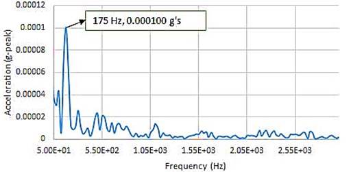
Similar to the acoustic experimentation, the g-peak acceleration values were measured for Machine C throughout the duration of 102 days, following the same experimental procedure as illustrated in Section 2. The last dates for both readings were the same. The coolant system was in continuous use while conducting the experiment. The main reason was to avoid excessive temperature rise during the cutting operations as well as to avoid tool damage and make the work on the lathe conducive to principles of production techniques. However, a completely isolated vibration signature of the coolant system was recorded while the lathe was not in use. The fundamental frequency corresponding to this coolant system was found to be equal to 175 Hz. The vibration signature for the same is shown in Fig. 4. Further analysis of results were carried out only after the fundamental frequency and all the harmonics of the coolant system were neglected from the signatures of the lathe machine for idle running, facing and turning.
Fig. 4Vibration signature of coolant system
The depth of cut and feed given were kept constant (at same values as mentioned above) for all the experiments. 300 frames were recorded by the accelerometer for each run and the results were captured and processed through the EDM software. The results obtained on some representative days are shown in Table 5.
Table 5g-peak training data for overall vibrations
S. No. | Day No. | Idle Run (g-peak) | Turning (g-peak) | Facing (g-peak) |
1. | 1 | 0.001671 | 0.00077 | 0.00257 |
2. | 6 | 0.002150 | 0.00108 | 0.00318 |
3. | 12 | 0.002630 | 0.00124 | 0.00375 |
4. | 21 | 0.003010 | 0.00169 | 0.00424 |
5. | 26 | 0.003450 | 0.00213 | 0.00496 |
6. | 34 | 0.003760 | 0.00245 | 0.00547 |
7. | 39 | 0.004060 | 0.00281 | 0.00603 |
8. | 46 | 0.004540 | 0.00302 | 0.00684 |
9. | 64 | 0.009500 | 0.00757 | 0.00937 |
10. | 102 | 0.012630 | 0.00985 | 0.01490 |
3.3. Headstock bearing vibration results
The vibrations of the headstock bearings can be qualitatively identified from the vibratory signatures of the overall lathe machine. The theoretical fundamental frequencies corresponding to the bearing parts [18] can be obtained from the relations given below:
where FTF – fundamental train frequency, BPFI – frequency of inner ring, BPFO – ball pass frequency of outer ring, – revolutions per second, – ball/roller diameter, – pitch diameter, – number of balls/rollers.
For our experiments, the bearing specifications and calculated frequencies are shown in Table 6.
Table 6Bearing specifications
Parameter | Value | Parameter | Value |
19 | (rev/s) | 30 | |
(mm) | 0.343 | 0° | |
(mm) | 3.543 | FTF (Hz) | 13.5478 |
(Hz) | 312.591 | BPFO (Hz) | 257.408 |
The vibration signatures of Machine C (for idle running, turning and facing operations) were scanned for g-peaks corresponding to calculated FTF, BPFI and BPFO. The overall vibration signature of the Machine C zoomed in the range 0 to 800 Hz is shown in Fig. 5. The peak at 175 Hz is to be neglected, as it corresponds to the coolant system as shown before. The next significant peak occurs at around 318 Hz as pointed out in Fig. 5. This falls around the theoretical value of BPFI. As there is no significant peak around the values of BPFO and FTF, we can establish that the outer race and the ball bearings unlike the inner race are in good condition. Further, the results of the g-peak values corresponding to a specific Day No. is tabulated in Table 7.
Fig. 5Overall vibration signature
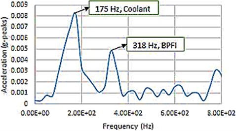
Table 7g-peak training data for bearing vibrations
S. No. | Day No. | Idle Run (g-peak) | Turning (g-peak) | Facing (g-peak) |
1. | 1 | 0.00056 | 0.00042 | 0.00075 |
2. | 6 | 0.00083 | 0.00049 | 0.00095 |
3. | 12 | 0.00121 | 0.00056 | 0.001295 |
4. | 21 | 0.00156 | 0.00061 | 0.001623 |
5. | 26 | 0.00196 | 0.00065 | 0.002012 |
6. | 34 | 0.00221 | 0.00069 | 0.002301 |
7. | 39 | 0.00250 | 0.00073 | 0.00256 |
8. | 46 | 0.002638 | 0.00076 | 0.00273 |
9. | 64 | 0.00412 | 0.001992 | 0.00325 |
10. | 102 | 0.004212 | 0.003088 | 0.00434 |
4. Predictive model and algorithm
Preventive maintenance [3-4] is a method which is carried out at regular time intervals irrespective of the indication or occurrence of a failure. In contrast, the Predictive method [3-4] involves scheduling maintenance or replacement of parts only when a functional failure is detected or predicted. The latter’s main advantage is that the monetary and other resources are judiciously used only when needed unlike the former.
The vibro-acoustic historical data of the lathe machine is the foundation for the development of a predictive model which can be achieved through machine learning algorithms [4-5, 19-21]. In this case, the predictive model is developed using two methods – Normal Equations Method and Artificial Neural Networks.
4.1. Normal equations method
In case of Normal Equations model, the historical data or the training set is fed to the learning algorithm which in turn assists a hypothesis function [22] to predict the number of days till the threshold value is reached at which the lathe needs maintenance.
The hypothesis function, developed is shown below:
where – idle run data, – turning data, – facing data. Each (1, 2, 3) may be the acoustic, vibratory or threshold value for which the is the corresponding value of Day No. The squared error function [22] is defined as shown below:
where is the value of the Day No. in the training set.
To estimate the threshold value of corresponding to the threshold values of the function has to be optimized to get the values of ( 1, 2, 3). Solving for optimal values of we get the Normal equation [22] which gives a closed form solution to the multi variate regression model:
where is the design matrix consisting of all and is the transpose of .
4.2. Artificial neural networks
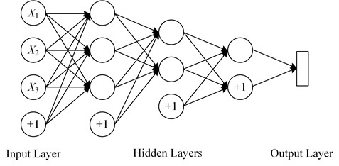
This section deals with the development of predictive models using Artificial Neural Networks (ANN) [19-20]. As opposed to the traditional mathematic and statistical models, ANN is a robust tool that can capture non-linear relationships with better accuracy and can automatically adjust their weights to optimize their behaviour. The basic architecture of every ANN consists of three layers-input layer, hidden layer and output layer.
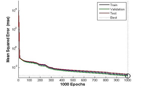
In our case, a Feedforward Backpropagation Neural Network model [19-20, 23-24] has been implemented for training and simulating the historical data. It has two layers of hidden network (Fig. 6) and is trained using the Levenberg-Marquardt algorithm. The input to the network is the training data obtained for Idle running, Turning and Facing operations and the output is the corresponding value of day number. The Mean Sqaured Error function is used as the performance function for performing input to output mapping with higher accuracy. Once the network is trained and the validation performance curve has reached its minima, the network is simulated using the threshhold values to obtain the number of days to failure.
For training the input data, all the neurons are sigmoidal in the three layered architecture. Any other activation functions have not been used because there was no need to worry about over fitting, given the amount of data we had. The number of layers in the neural networks was tuned as a hyper-parameter to the algorithm and the best results were obtained using the three layered structure. A ten fold cross validation set database was used. The application of both the algorithms has been explained in Section 5 for Acoustic and Vibration analysis.
Fig. 6Neural network architecture
5. Predictive analysis
5.1. Normal equation model
In order to develop the overall acoustic prediction model, the training set (157) shown in Table 4 is fed to the machine learning algorithm discussed in Section 4.1. The hypothesis function obtained by optimizing the squared error function is shown below:
The threshold values for are substituted from Table 3 to get the threshold value of which is the Day No. at which maintenance is to be carried out. A value of 156.69 is obtained by subtracting the duration of the experiment from the threshold value of . The significance of this value in the hypothesis function is discussed in Section 6. The overall vibration prediction model is developed using the training set ( 102) shown in Table 5 as input to the machine learning algorithm discussed in Section 4. The hypothesis function obtained by optimizing the squared error function is shown below:
Similar to the procedure mentioned before, the threshold values for are substituted from Table 3 to get the threshold value of which is the Day No. at which maintenance is to be carried out. A value of 164.66 is obtained by subtracting the duration of the experiment from the threshold value of . The significance of this value as well as the negative coefficient of in the hypothesis function is discussed in Section 6. In order to develop the vibration prediction model for the headstock bearings, the training set ( 102) shown in Table 7 is fed to the machine learning algorithm discussed in Section 4. The hypothesis function obtained by optimizing the squared error function is shown below:
The threshold values for are substituted from Table 3 to get the threshold value of which is the Day No. at which maintenance is to be carried out. A value of 178.59 is obtained by subtracting the duration of the experiment from the threshold value of . The significance of this value as well as the negative coefficient of in the hypothesis function is discussed in Section 6.
5.2. Artificial neural networks
In order to develop the overall acoustic prediction model, the acoustic training set shown in Table 4 is used as input to the network and the corresponding day number as output. The network is trained and the validation performance of 0.0011343 is achieved at 1000 epoch as shown in Fig. 7. The network is then simulated using the threshold values from Table 3 and a value of 153.0457 is obtained as output which is the day number at which maintenance is to be carried out.
In order to develop the overall vibration prediction model, the historical data shown in Table 5 is used to train the network. Best validation performance of 0.001389 is achieved at 1000 epochs as shown in Fig. 8. The network is then simulated using the threshold values from Table 3 and an output value of 164.5762 is obtained. Similarly, the vibration prediction model for the headstock bearings is developed using the training set shown in Table 7. Best validation performance of 0.00014865 is obtained at 1000 epochs as shown in Fig. 9. Using the threshold values as shown in Table 3, the network is simulated and an output value of 180.853 days is obtained. The significance of all these values is discussed in Section 6.
Fig. 7Performance curve for acoustic predictive model
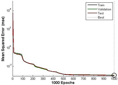
Fig. 8Performance curve for vibration predictive model
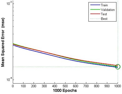
Fig. 9Performance curve for headstock bearing vibration predictive model
6. Discusion
6.1. Trends and results
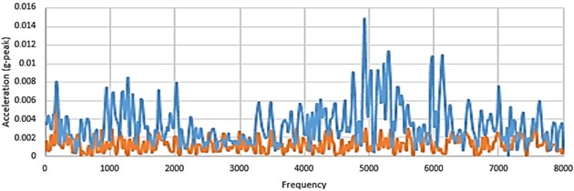
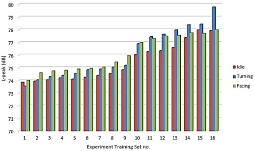
The following figures (Figs. 10-13) show the variation in the vibration signatures and acoustic level from the start to the end of experiment. The orange plot in Figs. 10, 11 and 12 is the vibration signature obtained at the start (Day 1) of the experiment wheras the blue plot shows the vibration signature obtained at the last day (Day 102) of the experiment. Fig. 13 shows us the increase in Decibel values over the entire duration of experiment for Idle Running, Turning and Facing operations. From the graphs it is clear that there is a general increase in the acceleration g-peak values and the -peak values over a period of time.
Fig. 10Vibration signature – Idle running
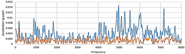
Fig. 11Vibration signature – Turning
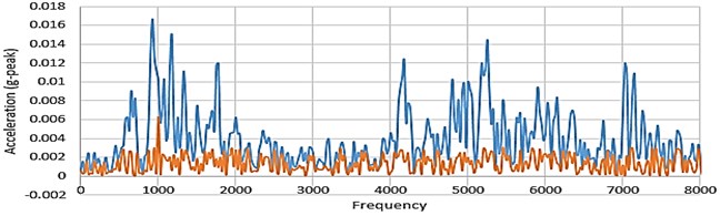
Fig. 12Vibration signature – Facing
6.2. Analysis of trends and inferences
The results obtained in Section 5 give us the duration after which the maintenance of Lathe and replacement of faulty parts needs to be carried out. For the overall acoustic prediction, the Normal Equations model and the Artificial Neural Networks model yield values 156.69 and 153.0457 days which signifies that if the prediction algorithms give these results today, then the next maintenance will be due in about 153 to 156 days from now. Hence, scheduling a maintenance on or before the 153rd day will probably prevent a possible breakdown of the machine. Firstly, the lesser value is taken here assuming that an earlier date is only reassuring the safety of the machine. Secondly, this inference is valid only for the lathe machine chosen in our experiment and the given training set. However, this procedure or prediction model can be applied to other lathe machines to predict failures or to schedule maintenance. Similarly, for the overall vibration prediction, the normal equations model and the ANN model give us values – 164.66 and 164.7 respectively which show the durations after which maintenance is to be scheduled. Again, these values signify that maintenance scheduled on or before the 164th day will probably prevent deterioration of the lathe. The values of 178.59 or 180.53 obtained from the two models discussed which is obtained from the bearing vibration analysis can be used as a good prediction of the no. of days till the next headstock bearing replacement for the lathe machine.
Fig. 13Acoustic signatures for all processes
In case of the Normal Equations method, a multi-variable model was used to build the prediction algorithm. However it must be noted that to visualize the effect of change of only one of the parameters in the multi-variable model, a new hypothesis function which includes only that parameter, i.e. a uni-variable model must be formulated. Hence, the negative coefficients of in the hypothesis functions in equations do not imply a negative dependence of with . For instance, in order to account for the dependence of only idle running operation on the prediction value, instead of substituting the values of variables and as null in the multi-variable model, we formulate a uni-variable model using the historical data so obtained for idle running. The uni-variable model formulated using the g-peak values to account for only idle running operation gives us the following form of the hypothesis function:
This shows that only if the dependence of more than one parameter is to be incorporated, a multi – variable model is adopted. Moreover, if it is needed to study the effect of only one parameter, for example the turning operation on the lathe machine’s performance, then it is incorrect to use a multi-variable model equation by inputting a null value for the other .
7. Conclusions
The vibro-acoustic condition monitoring of the lathe machine C allowed the development of two predictive models namely the Normal Equations method and the Artificial Neural Networks method. Each model has been used for two different approaches, one on the basis of the acoustic -peak values and the other on the basis of the characteristic vibration signatures and acceleration g-peak values. Both, the normal equation and the Artificial Neural Network methods provide very close results to the actual scheduling dates obtained from the workshop administration and the manufacturers, thereby validating the predictive model.
The overall vibration and overall acoustic signatures allow us to get a good estimate for scheduling regular overall maintenance of the Lathe machine. However, the bearing vibration signature is only indicative of the specific headstock bearing for which the historical data was collected, thereby giving us a safe date for maintenance of the bearing or probably even change of bearing.
Another aspect of the analysis is that acoustic results in general tend to give us a relatively earlier value or prediction. It is not feasible to carry out vibration testing without contact of the sensors and the surface of the headstock or the particular lathe machine part. However, it is possible to carry out this testing for acoustic structural health monitoring. In the acoustic approach, no parts need to be explicitly exposed unlike the vibration testing method. Moreover, no contact between surfaces and sensors is required in this case. Over and above such advantages, the acoustic method gives us a safer value than the reliable vibration condition monitoring. Hence, it can be safely taken that the acoustic method is also equally reliable to predict failure or to schedule maintenance of the lathe machine.
Both the models presented here are generic in nature but the training data provided is specific to the Lathe machine chosen for preparing the model. Hence, the training sets are not the main basis for the predictive models, instead the normal equations method and the ANN method are to be taken into consideration from a holistic point of view. Hence, if a predictive model is to be developed for a specific lathe machine, then new historical data will be required. However, the two generic methodologies discussed here can be adopted to any lathe machine having its own historical training data.
As the models have been developed in an open workshop and not in a closed laboratory environment, they can be designed for any machine in an industry. As mentioned, a separate table must be prepared similar to Table 1 and the threshold values should be obtained using the methods discussed above. To proceed with the development of the predictive model, each machine must have its own vibration and acoustic training data. This training data along with the threshold values can be further fed to the Normal Equation or the ANN algorithm to get a predicted date of failure. This will help in scheduling the maintenance of that particular machine based solely on its own historical data.
References
-
Martin K. F. A review by discussion of condition monitoring and fault diagnosis in machine tools. International Journal of Machine Tools and Manufacture, Vol. 34, Issue 4, 1994, p. 527-551.
-
Cempel Czeslaw Vibroacoustic condition monitoring. NASA STI/Recon Technical Report A, Vol. 93, 1991, p. 17525.
-
Scheffer Cornelius, Paresh Girdhar Practical Machinery Vibration Analysis and Predictive Maintenance. Elsevier, 2004.
-
Rao J. S. Vibratory Condition Monitoring of Machines. CRC Press, 2000.
-
Anderson John Robert Machine Learning: an Artificial Intelligence Approach. Vol. 2. Morgan Kaufmann, 1986.
-
De Silva Clarence W. Vibration Monitoring, Testing and Instrumentation. CRC Press, 2012.
-
Rangwala S., Dornfeld D. Sensor integration using neural networks for intelligent tool condition monitoring. Journal of Manufacturing Science and Engineering, Vol. 112, Issue 3, 1990, p. 219-228.
-
Farrar Charles R., et al. A review of structural health monitoring literature: 1996-2001. Los Alamos. Los Alamos National Laboratory, NM, 2004.
-
Swansson N. S. Application of vibration signal analysis techniques to condition monitoring. Conference on Lubrication, Friction and Wear in Engineering, Melbourne, Institution of Engineers, Australia, 1980.
-
Byrne G., et al. Tool condition monitoring (TCM) – the status of research and industrial application. CIRP Annals-Manufacturing Technology, Vol. 44, Issue 2, 1995, p. 541-567.
-
Jemielniak K. Commercial tool condition monitoring systems. The International Journal of Advanced Manufacturing Technology, Vol. 15, Issue 10, 1999, p. 711-721.
-
Nandi Subhasis, Hamid A. Toliyat, Xiaodong Li Condition monitoring and fault diagnosis of electrical motors – a review. IEEE Transactions on Energy Conversion, Vol. 20, Issue 4, 2005, p. 719-729.
-
Spider-81 Vibration Controller System Brochure. http://www.hzrad.com/pdf/Spider-81-Brochure.pdf.
-
Larson-Davis Noise Level Meter Model 831. http://www.larsondavis.com/products/soundlevelmeters/ Model831.aspx.
-
Sheng Xiaohong, Yu-Hen Hu Maximum likelihood multiple-source localization using acoustic energy measurements with wireless sensor networks. IEEE Transactions on Signal Processing, Vol. 53, Issue 1, 2005, p. 44-53.
-
www.formfonts.com
-
ShawBrian K., Richard S. McGowan, Turvey M. T. An acoustic variable specifying time-to-contact. Ecological Psychology, Vol. 3, Issue 3, 1991, p. 253-261.
-
Dyer D., Stewart R. M. Detection of rolling element bearing damage by statistical vibration analysis. Journal of Mechanical Design, Vol. 100, Issue 2, 1978, p. 229-235.
-
Samanta B., Al-Balushi K. R. Artificial neural network based fault diagnostics of rolling element bearings using time-domain features. Mechanical Systems and Signal Processing, Vol. 17, Issue 2, 2003, p. 317-328.
-
Su Hua, Kil To Chong Induction machine condition monitoring using neural network modeling. IEEE Transactions on Industrial Electronics, Vol. 54, Issue 1, 2007, p. 241-249.
-
Bishop Christopher M. Pattern Recognition and Machine Learning. Vol. 1. Springer, New York, 2006.
-
Chu Cheng, et al. Map-reduce for machine learning on multicore. Advances in Neural Information Processing Systems, Vol. 19, 2007, p. 281-288.
-
Hornik Kurt, Maxwell Stinchcombe, Halbert White Multilayer feedforward networks are universal approximators. Neural Networks, Vol. 2, Issue 5, 1989, p. 359-366.
-
PinedaFernando J. Generalization of back-propagation to recurrent neural networks. Physical Review Letters, Vol. 59, Issue 19, 1987, p. 2229-2232.
About this article
