Abstract
Long wavelength track irregularities are the key factors which influence vehicle stability and comfort. An on-line monitoring method is proposed to detect the vertical long wavelength track irregularities based on bogie pitch rate. Firstly, the principle of on-line monitoring method based on axle-box acceleration or bogie pitch rate was presented. Secondly, to process bogie pitch rate, a mix-filtering approach which contains time-space domain transformation, double integration, baseline correction and RLS (Recursive Least Squares) adaptive compensation filter was proposed. Thirdly, a coupling dynamics model of vertical vehicle-track interactions was developed to obtain bogie pitch rate. The obtained bogie pitch rate was then filtered with the signal processing approach. When the processed result compares with the actual irregularities, the SD (Standard Deviation) is 0.327 mm and the NMSE (Normalized Mean Square Error) is –9.1495. The experimental result shows that the proposed on-line monitoring method based on bogie pitch rate and signal processing approach are capable of monitoring the long wavelength track irregularities accurately and effectively.
1. Introduction
Track irregularities are track defects in geometry which caused by continuous wheel rail contact force and the deterioration of rail or sleeper. It is a main excitation source which causes vehicle and track vibration. It will influence the stability, comfort, wheel rail service life and even operational safety of rail transit [1]. Track irregularities can be divided into long wavelength irregularities and short wavelength irregularities in terms of wavelength, and the long wavelength track irregularities are the key factors which influence vehicle stability and comfort. Effective detection of the long wavelength track irregularities has great significance to railway operation.
Track irregularities are usually measured in displacement by a trolley measurement system that uses acceleration sensors with contact probes during maintenance work [2]. The contact probes have a speed limit during the measurement, so that this method can hardly be used to measure the long wavelength irregularities. Another method is adding testing equipment on the bottom of track inspection vehicle to record track irregularities after track inspection vehicle running through a specific area. The purchase and maintenance costs of track inspection car are high, and due to the needing for specialized schedule, it cannot realize monitoring the track condition in time. On-line monitoring track irregularities from an in-service vehicle allows for continual track monitoring so that both sudden and longer-term changes in track geometry can be detected [3-14]. This provides the possibility of timely maintenance intervention, avoids the need for more extensive maintenance at a later date, and allows degradation to be tracked.
A volume of research on online monitoring has been published. Optical method [3] basically consists of a laser scanner which determines the rail profile. This method is currently widely employed as it is faster and can measure longer rail defects with reduced wear. Nevertheless, the optical method is expensive and keeping optical sensors working in the dirty railway environment is challenging.
Apart from the optical methods, there is another non-contact technique based on inertial methods which tries to determinate track irregularities by measuring displacement, accelerations or angle velocity. L. Chong [4] installed inertial strap-down system in car body to monitor the long wavelength irregularities of the maglev rail. However, it is difficult to specifically evaluate track irregularities without considering the influence from the primary and secondly suspension. AEAT’s Track-Mon system [5] uses vertically sensing accelerometers on the bogie plus vertically sensing displacement transducers to measure down from the bogie to the left and right axle-boxes. Tsunashima H. et al. [6] summarized the track-condition-monitoring system for conventional and high speed railway used in Japanese railway. For conventional railway, rail irregularities are estimated from the vertical and lateral acceleration of the car body. The roll angle of the car body, calculated using a rate gyroscope, is used to distinguish line irregularities from level irregularities. For high speed railway, track condition monitoring that only references car body accelerations become difficult because the high speed vehicle is equipped with high-performance suspension. Therefore, the track condition monitoring system for high speed railway used double integration of the axle-box acceleration to measure vertical track irregularities.
The assessment of track irregularities has also been regarded as a process of inverse model identification by some authors. These research usually focused on taking multi-signal into account, developed a theoretically simulation model at first, then constructed a inverse model to monitor track irregularities. Alfi S. et al. [7] proposed a method for the estimation of track irregularities having wavelength above 20 m based on car-body attached acceleration, bogie attached acceleration and axle-box attached acceleration. Measurements are fed into a model-based identification procedure in which the input-output relationship between track irregularity and vehicle dynamics is reversed to achieve track irregularity reconstruction. Even the track irregularities can be solved accurately, the shortage of this method is the difference between the dynamic model and real railway operation. The track is treated in a simple way without the consideration of nonlinear track-vehicle interaction and the flexibility of track. In contrast, Li M. X. D. et al. [8] developed a more detailed wheel-rail dynamic model which is composed of track, vehicle, and wheel-rail contacting with moving irregularities. By solveing it in the frequency domain with fast Fourier transform or in the time domain by constructing a filter function based on system identification, vertical track geometry can be assessed. This research is mainly focused on theoretical model, while less research is regarded real time online monitoring system. Furthermore, Uhl T. et al. [9] proposed a SHM system based on vibration measurements during the rail vehicle operation simultaneously with GPS position and velocity estimation. Algorithm for rail track health assessment is formulated as inverse identification problem of dynamic parameters of rail-vehicle system. By this procedure, track irregularities are identified. Another interesting work was done by Song Liu et al. [10]. They constructed an inverse system by NARX neural network to predict track irregularities, in which the input is the vibration of vehicle body and the output is track irregularities.
The main problem with inertial methods is data manipulation. If realistic results are to be obtained, accelerations must be filtered or processed for the elimination of some base components that introduce important errors in the integration process. This manipulation process may become very complex and problematic for the required accuracy of the results. As a matter of fact, J. Real et al. [11] and Lee et al. [12] proposed different ways of solving this. In literature of J. Real, the axle-box mounted acceleration signal is processed by a filtering approach, based on dynamic interaction model, double integration, high-pass filter and phase correction filter, to estimate the track irregularities. In literature of Lee, with track geometry measurement system, the axle-box and bogie mounted acceleration is processed by a filtering approach including kalman filter, band-pass filter, and compensation filter to estimate the track irregularities. As a direction of further research in data processing, Long Q. et al. [13] designed an onboard track fault diagnosis device for advanced railway condition monitoring. Track faults are diagnosed from the vertical and lateral acceleration of axle-box, bogie and car-body with different characteristics. The algorithm first transformes the vibration signal into frequency-domain, then calculating probabilities of fault tracks with PCA and SVM, applying D-S evidence theory to fuse multi-source information at last.
A practically complete research that deals with both experimental set-up and data processing is made by Weston et al. [14]. Used sensors are a bogie-mounted pitch rate gyro to obtain mean vertical alignment and axle-box accelerometers to calculate the defects wavelength. In this way, wavelengths from 5 to 70 m are analysed. Axle-box accelerators may be used if shorter wavelengths need to be monitored. For longer wavelengths, these authors originally claim that the long wavelength irregularity presents accelerations that are a fraction of 1 g, and so the axle-box accelerator sensor has to have a low limit on lower bandwidth, high linearity, and very low noise to provide usable long wavelength results.
This article aims to propose the use of a bogie-mounted pitch-rate gyro to detect vertical long wavelength track irregularities. Using this sensor alone provides a large amount of advantages such as low cost and a good engineering applicability. Section 2 analyses the principle of on-line monitoring method based on axle-box acceleration or bogie pitch rate. Section 3 proposes a mix-filtering approach to process bogie pitch rate. Section 4 develops coupling dynamics model of vertical vehicle-track interactions. Section 5 uses actual measured irregularities as model excitation to obtain simulation data of bogie pitch rate. The obtained bogie pitch rate was then filtered by mix-filtering approach in this section and the result has been compared with the actual measured irregularities.
2. Principle of on-line monitoring
This section analyzes the principle of on-line monitoring method based on axle-box acceleration or bogie pitch rate. And then bogie pitch rate is selected to detect the long wavelength irregularity.
2.1. Sensor installation
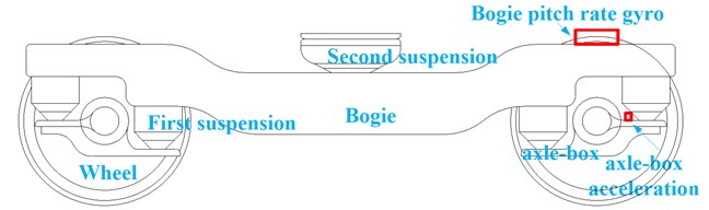
Piezoelectric accelerometer and gyroscope are widely used so that on-line monitoring of track irregularities can be realized by detecting axle-box acceleration and bogie pitch rate etc. An axle-box piezoelectric accelerometer and bogie pitch gyroscope are mounted on an operational vehicle as shown in Fig. 1. The gyro is located above axle-box. And that mounting the sensor in the same location on the other side of bogie can constitute a whole system to monitor both left and right vertical track irregularities.
Fig. 1Mounting position of an axle-box piezoelectric accelerometer and bogie pitch gyroscope
2.2. Axle-box acceleration
Axle-box acceleration is typically turned into displacement information by double integration of the signal with respect to time:
where is displacement along the track (m), is axle-box acceleration (m/s2), is vehicle speed along track(m/s), is the acceleration sampling time, is the estimation of acceleration-derived vertical position (m).
The double integration results in the well-known effect of not just drift, but integrated drift, that has to be filtered out by filtering out long wavelength results [14]. The signal of axle-box acceleration also contains ingredients such as rolling bearing fault, wheel tread fault, wheel and rail out of contact and environmental noise, etc. [15]. Each of them will bring certain interference to the process of information extraction.
When the train passes through short track defects like squats, welds with poor finishing quality, insulated joints and corrugation etc, axle-box accelerometers response accelerations as high as 100 g [16]. However, the long wavelength irregularities presents accelerations that are a fraction of 1 g, so the sensor has to have a low limit on lower bandwidth, high linearity and very low noise to provide usable long wavelength results [14].
2.3. Bogie pitch rate
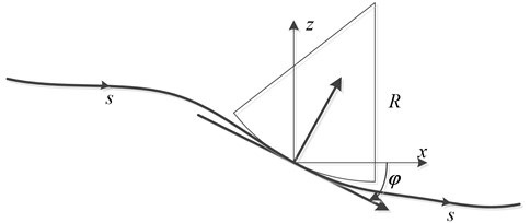
In Fig. 2, let a bogie pitch-rate gyro be oriented an angle velocity . If the pitch angle of the rate gyro is approximately equal to the pitch angle of the track, then an estimate for the corresponding vertical displacement is given by:
where is displacement along the track (m), is pitch angle (rad), is vehicle speed along track (m/s), is the estimation of pitch-rate gyro-derived vertical position (m).
Fig. 2Wheelrail contact diagram
Bogie pitch rate with respect to the ‘pitch’ of the track depends on the bogie wheelbase, the primary and secondary suspension.
Assuming that the leading and trailing wheel-sets follow the vertical track geometry and the primary suspension is infinitely stiff, the bogie pitch is determined by the vertical positions of the leading and trailing wheel-sets divided by the bogie wheelbase. The relationship between bogie pitch and track vertical geometry is given by a geometric filter (spatial filtering) in which the bogie pitch is blind to irregularities at wavelengths equal to the bogie wheelbase. For wavelengths longer than 8 m, the bogie pitch follows the mean track slope fairly accurately (unit gain), the gain falling to-3 dB around 4 m (for a bogie wheelbase of 2.5 m), then rapidly falling to zero gain at 2.5 m wavelengths. The suspension system allows the bogie pitch to have additional movement relative to the instantaneous track slope between the wheelsets on the bogie.
The primary vertical suspension and bogie pitch inertia combine to allow a bogie pitch resonance, typically at a frequency of around 12 Hz. This corresponds to a wavelength of close to 4 m at 45 m/s, which is about the same wavelength as that where the bogie pitch is becoming blind to the track geometry. At lower vehicle speeds, the wavelength corresponding to the pitch resonance is less than 4 m and the geometric filtering is more important. The secondary suspension configuration determines the effect of the secondary suspension on the bogie pitch motion. If the secondary vertical suspension components are longitudinally symmetric about the center-line of the bogie, body bounce above the bogie does not generate significant bogie pitch motion.
3. Mix-filtering approach for bogie mounted pitch rate
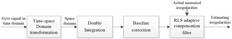
From Eq. (2) the vertical track irregularities can be estimated by double integration of the signal with respect to space domain. During the process of observation, the gyroscope output contains two types of errors which will influence irregularity estimation. One is Gaussian noise caused by environment vibration or electromagnetic radiation. The other is installation error caused by the sensitive axis of sensor not completely perpendicular to the plane of the train running line. Installation error is a constant proportion. Taking the bogie pitch observation error and the sensor signal characteristics into account, a mix-filtering approach for processing gyro signal in time domain is proposed to estimate track irregularities as shown in Fig. 3. This mix-filtering approach use bogie pitch gyro signal and vehicle speed signal as input. It contains 4 steps including time space domain transformation, double integration, baseline correction and RLS adaptive compensation filter.
Fig. 3Mix-filtering approach
Step1: Time-space domain transformation
The output of bogie mounted pitch rate gyro in time domain is obtained while vehicle is online operation. The relationship between and is as follows:
where is the sampling time; is the spatial interval. Thus, the time-space domain transformation by the use of vehicle speed along track is .
Step 2: Double integration filter
There are methods, such as immediate integration, frequency conversion method and filter method etc, to realize signal integration. The immediate integration and frequency conversion method cannot realize continuous calculation. Therefore, the filter method is used. Transfer function of double integral filter derived by the rectangular integration as below [17]:
where and are spatial interval of 2 th, 1th and th sampling points, respectively.
Step 3: Baseline correction
Although integration filter process seems to be straightforward, some difficulties must be corrected to avoid results distortion. These difficulties come from reduction of high-frequency contents of the waveform, amplification of low frequencies and signal phase shift. The signal of pitch rate gyro contains observation noise , so that the numerical integration will produce a constant term (zero frequency term) and a linear term (second integration time), these trends items must be eliminated.
There are different methods used to improve velocity and displacement calculated diagrams such as high-pass filter method and wavelet transform method [18]. A widely used technique is the so-called ‘baseline correction’ [11]. This procedure consists of defining a baseline function that fits the data of the diagram by least squares method. Initial condition -zero velocity at initial instant- must be satisfied.
Chosen baseline function is a sixth degree polynomial. The recursive computation is as follows [19]:
where is the polynomial order degree, is the number of observations, is the observation data. According to Eq. (5), before knowning number of observation data sequence , the and can be obtained, and then , , and can be derived as well. Finally, the baseline corrected observations can be obtained using equation .
Step 4: RLS adaptive compensation filter
It is well known that the relationship between bogie pitch rate and vertical track irregularities is dependent on the sensor installation error, rail elasticity change, wheel-rail contact relationship and suspension characteristics. In addition, a signal takes a certain amount of time to pass through a filter, which leads to a change in the transmission phase angle with respect to the frequency, called the phase delay.
A compensation filter that uses a FIR (Finite Impulse Response, FIR) filter with adjustable parameters is proposed. It is described as follows:
where is the transfer function of the compensation filter. It is very difficult to identify these parameters by analytical methods because several different kinds of mechanisms are simultaneously involved. Instead of using analytic methods, an adaptive filtering method based on an RLS algorithm with the measured data is proposed.
The recursive computation of the filter parameters is as follows [20]:
where is input irregularities after baseline corrected, is the actual measured irregularities, is the filter parameter vector, is a forgetting factor in the range of 01. In Eq. (6), and are initialized by setting and . RLS algorithm is superior to LMS algorithm in convergence speed, stability and practicality of non-stationary signals. RLS’s shortcoming is a larger computational cost.
4. Numerical simulation model
A coupling dynamics model of vertical vehicle-track interactions is developed to obtain simulation data of bogie pitch rate. The model uses the actual measured long wavelength irregularities as excitation.
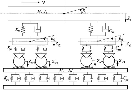
Coupling dynamics model of vertical vehicle-track interactions developed by Zhai [21] is a theoretical tool to research vertically vehicle-track discrete point dynamic interaction. Fig. 4 illustrates the various components of the vehicle–track model in which subsystems describing the vehicle and the track are spatially coupled by the wheel-rail interface.
By using the system of coordinates moving along the track with vehicle speed, the equations of motion of the vehicle subsystem can be derived according to D’Alembert’s principle, which can be described in the form of second-order differential equations in the time domain:
where is the mass matrix of the vehicle; and are the damping and the stiffness matrices which can depend on the current state of the vehicle subsystem to describe nonlinearities within the suspension; , and are the vectors of accelerations, velocities and displacements of the vehicle subsystem, respectively; is the system load vector representing the non- linear wheel-rail contact forces determined by the wheel-rail coupling model. The specific parameters see literature [21].
Fig. 4Coupling dynamics model of vertical vehicle-track interactions
The rail is treated as continuous Bernoulli-Euler beams which are discretely supported atrial-sleeper junctions by springs and dampers, representing the elasticity anddamping of the sleeper, respectively. The differential equation of vibration is:
where represents contact forces at the th wheel-contacting point; and are the elasticity anddamping of the sleeper, respectively; is the number of discrete support; is the modal order of the rail; is normalized coordinate of modal shape of the rail; is the elastic modulus of rail; is the cross-sectional rotational inertia of rail; is the length of rail; is the rail mass per unit length; is vibration mode function of rail which is:
The solution of Eq. (6) is the vertical track displacement:
is the displacement of the th wheel/rail vertical compression:
where is vertical displacement of the wheel; is vertical displacement of the rail; is the vertical irregularity of rail in th place at time .
The nonlinear Hertz elastic contact theory is used to calculate the wheel-rail normal contact forces which depends on the displacements of wheels and rails:
where 3.86-0.115×10⁻⁸ is the Hertz spring stiffness; is the radius of wheel.
In order to enhance the computational speed for dynamic system, a simple fast explicit integration method previously developed by Zhai is employed [21]. The main solution procedure for the vehicle–track coupled dynamics consists of the following four steps: estimating the displacement and the velocity of the system; calculating the acceleration computing the displacement and the velocity by using Newmark- equation; calculating the final acceleration .
5. Experiment
In this section, the coupling dynamics model is excited by a segment of actual measured irregularities from high-speed rail in china. The obtained bogie pitch rate was filtered with mix-filtering approach and the result has been compared with the actual measured irregularities.
5.1. Data preparation
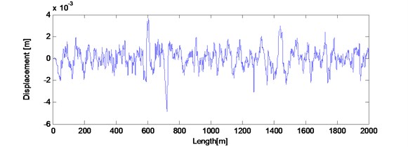
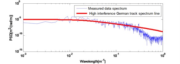
The track irregularities data is measured as a discrete sample sequence with 0.5 m intervals and the length of the data is 2 km. Fig. 5 plots the space waveform (a) and power spectra (b) of the measured data. The space waveform shows the amplitude of this segment irregularity data is less than 5 mm. Fig. 5(b) also plots the high interference German track spectrum line. By comparing with each other, this segment data contains irregularities of 6-300 m wavelength.
Coupling dynamics model has been numerically solved to obtain bogie pitch rate response by using actual measured long wavelength track irregularities as model excitation. Since the actual measured irregularities are discrete sample sequence with 0.5 m intervals, cubic spline interpolation has used for the data to obtain data with space step 0.001 m. During the process of simulation, the speed of train was set in 20 m/s, the size of space step 0.001 m, the iteration time 0.05 ms.
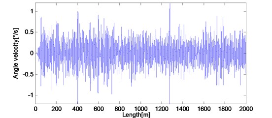
Fig. 6 shows the obtained bogie pitch rate . In this figure, bogie pitch rate responds in a range of 1°/s when detecting long wavelength irregularities. Comparing with 0.03°/s excited by broad gauge joint as shown in Fig. 5, the pitch rate only have one order of higher magnitude. Therefore, when detecting long wavelength irregularities, the bogie pitch rate is slightly affected by local irregularity. Nowadays, the resolution of fiber optic gyroscope is less than 10°/h, which can up to (1-5)°/h, so that it is able to meet the detecting requirements. This method can be implemented and has a good engineering applicability.
Fig. 5Actual measured long wavelength track irregularities: a) space waveform; b) power spectrum compared with high interference Germany track spectrum
a)
b)
Fig. 6Bogie pitch rate βt1 response of actual measured long wavelength track irregularities
The condition of simulation process is usually ideal, so the obtained bogie pitch rate data as shown in Fig. 7 has been multiplied by the coefficient 0.9 and added with a gauss noise sequence which variance 0.001 rad/s to simulate installation error and observation noise, respectively.
5.2. The mix-filtering of bogie pitch rate
To numerically evaluate the closeness of estimation between the filtered result and the actual displacement, we calculate SD (Standard Deviation) and NMSE (Normalized Mean Square Error) as follows:
where, is the error sequence of the filtered result and the actual measured displacement; is the mean value of :
where, is the actual measured displacement; is the filtered result.
Firstly, to convert into spatial domain, bogie pitch angular velocity was divided by the vehicle speed 20 m/s. Secondly, double integration filter was applied to obtain vertical track displacement. Then six degree of polynomial baseline correction iteration was applied to eliminate trends. In the processing of baseline correction, the number of calculating data 1000.
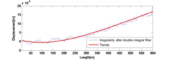
Fig. 7a) Results after double integral filter and trends extracted by 6 degree polynomial correction; b) the spatial irregularity waveform after double integral filter and six degree polynomial baseline correction compared with actual measured irregularities waveform
a)
b)
Results after the double integration filter and trends extracted by 6 degree polynomial correction are shown in Fig. 7(a). Results after trends eliminated and the actual measured irregularities are shown in Fig. 7(b). Fig. 7 (a) shows polynomial baseline correction method eliminates most of the trends. Fig. 7(b) shows the spatial waveform of the filtered result and the actual measured displacement. After double integration filter and six degree polynomial baseline correction, the 0.856 mm, the –0.8013. The filtered result has been close to the actual waveform, but still need compensated by compensation filter processing.
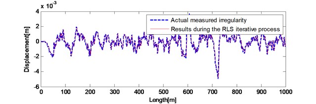
Spatial step of track irregularity data is 0.001 m and the actual effective wavelengths are longer than 3 m. Therefore, the built compensation filter has low-pass characteristic. In the processing of compensation, due to the filter length will affect the calculation speed of RLS adaptive algorithm, the number of adjustable parameters of the FIR filter model is set at 40. The parameter values are determined via recursive computation. The parameters are obtained from the RLS algorithm at the end of the front 1 km iteration and validated using last 1 km irregularity.
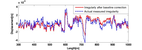
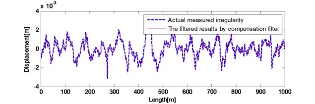
Results of the front 1km during the iterative process and the actual waveform are shown in Fig. 8(a). The filtered results of last 1 km by compensation filter and the actual waveform are shown in Fig. 8(b). After compensation filter, the 0.327 mm, the –9.1495. The filtered waveform in spatial domain is perfectly close to the actual waveform. The error between irregularity after baseline correction and the actual measured irregularities has been improved. Therefore, the irregularity obtained by filtering bogie pitch angular velocity with the mix-filtering approach reproduces the actual measured long wavelength track irregularities accurately and effectively.
Fig. 8Results compared with actual measured irregularities a) front 1 km during the iterative process; b) last 1 km after compensation filter
a)
b)
Fig. 9Results compared with actual measured irregularities in power spectrum
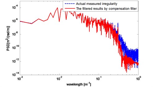
Power spectrum waveform of the actual measured 1 km data and data after the compensation filter in Fig. 8(b) is shown in Fig. 9 by welch method. When the wavelength is larger than 6 m (1/10-0.8), the reproduced harmonic components by bogie pitch rate method are consistent with the actual data. When the wavelength changing from 6 m to 2.5 m (1/10-0.4), harmonic components decreased approximately 2 dB. When the wavelength is between 2.5 m and 1 m (1/100) that means it is closed to the wheelbase, the harmonic components were dropped by 2 dB. Furthermore, when the wavelength is 1.6 m (1/10-0.2), there is no significant resonance occurring on the 12 Hz resonance point of first suspension while the speed of vehicle is 20 m/s.
In summary, after mix-filtering approach for bogie mounted pitch rate, the estimated track irregularities reproduce the long wavelength track irregularities accurately and effectively.
6. Conclusions
The use of a bogie-mounted pitch-rate gyro for detecting vertical long wavelength track irregularities was proposed. Using this sensor alone provides a large amount of advantages such as low cost and a good engineering applicability. A mix-filtering approach for bogie pitch rate was proposed. Coupling dynamics model of vertical vehicle-track interactions was developed to obtain simulation data of bogie pitch rate. The model uses actual measured irregularities as excitation. The obtained bogie pitch rate was filtered with mix-filtering approach. By comparing with the actual irregularities, the result shows the proposed bogie pitch rate based method and mix-filtering approach are capable of monitoring long wavelength track irregularities accurately and effectively. This method and mix-filtering approach are worth popularizing in engineering.
References
-
Shi Hongmei Research on Intelligent Sensing Algorithm of Track Irregularity Based on Vehicle Dynamic Rsesponses. Beijing Jiaotong University, 2012, (in Chinese).
-
Deshui Zhang Measurement of Railway Irregularities and Signal Processing. Shanghai Jiao Tong University, 2012, (in Chinese).
-
Molina L. F., Resendiz E., Edwards J. R., et al. Condition monitoring of railway turnouts and other track components using machine vision. Transportation Research Board 90th Annual Meeting, 2011.
-
Li Chong Real-Time Detecting and Processing of Track Long Wave Irregularities of Meglav Railway. Southwest Jiaotong University, 2006, (in Chinese).
-
Gilbert D., Wesley P. D. Track monitoring equipment. EU Patent EP1180175, 2002.
-
Tsunashima H., Kojima T., Matsummoto A., Mizuma T. Condition monitoring of railway track using in-service vehicle. Japanese Railway Engineering, Vol. 161, 2008, p. 333-356.
-
Alfi S., Bruni S. Estimation of long wavelength track irregularities from on board measurement. 4th IET International Conference on Railway Condition Monitoring, Stevenage, United Kingdom, 2008.
-
Li M. X. D., Berggren E. G., Berg M. Assessment of Vertical Track Geometry Quality Based on Simulations of Dynamic Track-Vehicle Interaction. Professional Engineering Publishing Ltd., London, United Kingdom, 2009.
-
Uhl T., Mendrok K., Chudzikiewicz A. Rail track and rail vehicle intelligent monitoring system. Archives of Transport, Vol. 22, Issue 4, 2010, p. 496-510.
-
Liu S., Pang X., Ji H., Chen H. Prediction of track irregularities using NARX neural network. Second Pacific-Asia Conference on Circuits, Communications and System (PACCS), 2010.
-
Real J., Salvador P., Montalbán L., et al. Determination of rail vertical profile through inertial methods. Proceedings of the Institution of Mechanical Engineers, Part F: Journal of Rail and Rapid Transit, Vol. 225, Issue 1, 2011, p. 14-23.
-
Lee J. S., Choi S., Kim S. S., et al. A mixed filtering approach for track condition monitoring using accelerometers on the axle box and bogie. IEEE Transactions on Instrumentation and Measurement, Vol. 61, Issue 3, 2012, p. 749-758.
-
Long Q., Wei D., Yanbo S. Design of onboard device to diagnose track fault online. Applied Mechanics and Materials, Vol. 483, 2014, p. 465-470.
-
Weston P. F., Ling C. S., Roberts C., et al. Monitoring vertical track irregularity from in-service railway vehicles. Journal of Rail and Rapid Transit, 2007, p. 75-88.
-
Ning Jing, Zhu Chang Qian, Zhang Bing An approach for signal analysis of track irregularity based on EMD and Cohen’s kernel. Journal of Vibration and Sound, Vol. 4, 2013, p. 31-38, (in Chinese).
-
Marija Molodova, Zili Li, Rolf Dollevoet Axle box acceleration: Measurement and simulation for detection of short track defects. Wear, Vol. 271, Issue 1-2, 2011, p. 349-356.
-
Zheng Shubin, Lin Jianhui, Li Guobin Design of track long wave irregularity inspection system for high speed maglev. Chiness Journal of Scientific Instrument, Vol. 28, Issue 10, 2007, p. 1781-1786, (in Chinese).
-
Yang Wengzhong, Lian Songliang Comparison of methods for removing trend in axle-box acceleration measured by railway track inspection car. Journal of Shijiazhuang Railway Institute, Vol. 2008, Issue 9, 2008, p. 9-13, (in Chinese).
-
Yang Shuzi, Wu Ya Time Serious Analysis in Engineering Application. Huazhonguniversity of Science and Technology Press, 2007, (in Chinese).
-
Zhang Linghua, Zheng Bayou Random Signal Processing. Tsinghua University Press, Beijing, 2003, (in Chinese).
-
Zhai W., Wang K., Cai C. Fundamentals of vehicle–track coupled dynamics. Vehicle System Dynamics, Vol. 47, Issue 11, 2009.
About this article
This research was carried out under independent project RCS2014ZT24 from State Key Lab of Traffic Control and Safety and Doctoral Scientific Fund Project 20120009110035.
