Flow noise computation and tail wing optimization of the underwater vehicle based on computational fluid dynamics

Zhang, Hongxin; Duan, Kanghong

Journal of Vibroengineering

Browse Journal

Submit article

Published: 15 August 2015

Check for updates

Flow noise computation and tail wing optimization of the underwater vehicle based on computational fluid dynamics

Hongxin Zhang¹

Kanghong Duan²

^{1, 2}North China Sea Marine Technical Support Center, Qingdao, 266033, China

Corresponding Author:

Hongxin Zhang

Cite the article Download PDF

Downloads 1188

Abstract

In this paper, the underwater vehicle was selected as the research object. Based on Computational Fluid Dynamics (CFD), the unsteady numerical simulation was carried out on the turbulent filed at different stream velocities. Then, the sound source was extracted according to the computational result of the flow field. The flow field and the flow noise of the underwater vehicle were computed by Lighthill acoustic analogy theory and FW-H equation, which were consistent with the experimental results, indicating that the computational method employed was effective. It could be obtained from the computational results that the tail wing had a great influence on the flow noise of the underwater vehicle. Consequently, to reduce resistance and noise, the traditional cross-shaped tail wing was changed into the symmetrically-arranged X-shaped tail wing which was 45° with the transverse and longitudinal sections of the underwater vehicle. Then, the simulation on the resistance and flow noise of the improved X-shaped tail wing was conducted. And the results showed that the blocking effect of the flow field by the improved X-shaped was weaker than that by the traditional cross-shaped. In addition, the flow noise of X-shaped tail wing was improved at a certain extent. However, the improvement was not very obvious. Therefore, this paper attempted to research the position and local shape of X-shaped tail wing in order to further optimize the radiation noise.

1. Introduction

In recent years, in order to make reasonable and reliable evaluation on the dynamic performances of the underwater vehicle and raise improvement methods in time, a large number of scholars [1-4] have employed CFD method to compute the flow field around the underwater vehicle, and have achieved certain progress. Zhang [5] computed the resistance and the wake field of two types for the underwater vehicle models by means of solving the RANS equation.

Among the published papers, the characteristics of the flow noise were mainly obtained through the experimental analysis. In reference [6], the time-domain signal of the flow noise for the underwater vehicle was obtained through the self-propulsion model experiment with effective signal processing method. The numerical simulation research on the flow noise started relatively late. Most of the early researches were focused on the computation method explorations, and simulation computation in engineering rarely emerged. Wang [7] numerically studied the far field sound in the boundary layer of the flat plate with low Mach number. Piomelli [8] studied the influence of micro-scale in Lighthill acoustic analogy. Bastin [9]researched on the numerical computation methods of the jet noise.

From the mentioned researches, it could be obtained that the numerical simulation of the flow noise can be conducted with certain computation accuracy based on Lighthill acoustic analogy theory. Therefore, in this paper, Reynolds Average Navier-Stokes equation (RANS) with turbulence model and FW-H acoustic model were employed to compute the flow field and the flow noise of the underwater vehicle. It could be obtained from the computational results that the tail wing had a great influence on the flow noise of the underwater vehicle. Consequently, to reduce resistance and noise, the traditional cross-shaped tail wing was changed into the symmetrically-arranged X-shaped tail wing which was 45° with the transverse and longitudinal sections of the underwater vehicle. Then, the numerical simulation on the resistance and flow noise of the improved X-shaped tail wing was conducted. And the results showed that the blocking effect of the flow field by the improved X-shaped was weaker than that by the traditional cross-shaped. In addition, the flow noise of X-shaped tail wing was improved at a certain extent. However, the improvement was not very obvious. Therefore, this paper attempted to research the position and local shape of X-shaped tail wing in order to further optimize the radiation noise.

2. Basic theory and mathematical model

2.1. Control equation and turbulence model

Continuity equation of the incompressible fluid is expressed as follows:

1

ρ \frac{\partial {\bar{u}}_{i}}{\partial t} + ρ {\bar{u}}_{i} \frac{\partial {\bar{u}}_{i}}{\partial x_{j}} = - \frac{\partial \bar{p}}{\partial x_{i}} + μ \frac{\partial^{2} {\bar{u}}_{i}}{\partial x_{j} \partial x_{j}} - ρ \frac{\partial {\bar{u}}_{i}^{'} {\bar{u}}_{j}^{'}}{\partial x_{i}} + ρ {\bar{f}}_{i} .

RANS equation can be expressed as follows:

2

ρ \frac{\partial {\bar{u}}_{i}}{\partial t} + ρ {\bar{u}}_{i} \frac{\partial {\bar{u}}_{i}}{\partial x_{j}} = - \frac{\partial \bar{p}}{\partial x_{i}} + μ \frac{\partial^{2} {\bar{u}}_{i}}{\partial x_{j} \partial x_{j}} - ρ \frac{\partial {\bar{u}}_{i}^{'} {\bar{u}}_{j}^{'}}{\partial x_{i}} + ρ {\bar{f}}_{i} .

The Reynolds average velocity:

\frac{\partial (ρ ε)}{\partial t} + \frac{\partial (ρ ε u_{j})}{\partial x_{j}} = \frac{\partial}{\partial x_{j}} [α_{k} μ_{e f f} \frac{\partial ε}{\partial x_{j}}] + C_{1 ε}^{^{*}} \frac{ε}{κ} C_{k} - C_{2 ε} ρ \frac{ε^{2}}{κ} .

Fluctuation velocity:

\frac{\partial (ρ ε)}{\partial t} + \frac{\partial (ρ ε u_{j})}{\partial x_{j}} = \frac{\partial}{\partial x_{j}} [α_{k} μ_{e f f} \frac{\partial ε}{\partial x_{j}}] + C_{1 ε}^{^{*}} \frac{ε}{κ} C_{k} - C_{2 ε} ρ \frac{ε^{2}}{κ} .

And ‘Reynolds Stress’:

\frac{\partial (ρ ε)}{\partial t} + \frac{\partial (ρ ε u_{j})}{\partial x_{j}} = \frac{\partial}{\partial x_{j}} [α_{k} μ_{e f f} \frac{\partial ε}{\partial x_{j}}] + C_{1 ε}^{^{*}} \frac{ε}{κ} C_{k} - C_{2 ε} ρ \frac{ε^{2}}{κ} .

It could be seen from RANS Eq. (2) that the Reynolds stress item – $ρ u_{i} u_{j}$ is a new unknown function. To close the equations, the assumption of Reynolds stress must be made. According to the different treatments on Reynolds stress, the turbulence model commonly included the following types which were the Reynolds stress equation model, the standard $k$ - $ε$ turbulence model, the RNG $k$ - $ε$ turbulence model and the $k$ - $ω$ turbulence model, respectively. In this paper, the RNG $k$ - $ε$ turbulence model was adopted.

In the RNG $k$ - $ε$ turbulence model, the influence of micro-scale was displayed through the large scale movements and the modified viscosity item, and then these micro-scale movements were removed from the control equation. After that, the $k$ equation and $ε$ equation were obtained as follows:

3

\frac{\partial (ρ ε)}{\partial t} + \frac{\partial (ρ ε u_{j})}{\partial x_{j}} = \frac{\partial}{\partial x_{j}} [α_{k} μ_{e f f} \frac{\partial ε}{\partial x_{j}}] + C_{1 ε}^{^{*}} \frac{ε}{κ} C_{k} - C_{2 ε} ρ \frac{ε^{2}}{κ},

4

\frac{\partial (ρ ε)}{\partial t} + \frac{\partial (ρ ε u_{j})}{\partial x_{j}} = \frac{\partial}{\partial x_{j}} [α_{k} μ_{e f f} \frac{\partial ε}{\partial x_{j}}] + C_{1 ε}^{^{*}} \frac{ε}{κ} C_{k} - C_{2 ε} ρ \frac{ε^{2}}{κ} .

2.2. Lighthill acoustic analogy theory

Lighthill equation can be described as follows [10]:

5

\frac{\partial^{2} ρ'}{\partial t^{2}} - c_{0}^{2} \nabla^{2} ρ^{'} = \frac{\partial^{2} T_{i j}}{\partial y_{i} \partial y_{j}},

where $T_{i j} = ρ u_{i} u_{j} - e_{i j} + δ [(p - p_{0}) - c_{0}^{2} (ρ - ρ_{0})]$ is the Lighthill turbulence stress tensor. $e_{i j}$ is the viscosity stress tensor. $p_{0}$ and $p$ are the fluid pressure intensity before and after the disturbance, respectively. $ρ' = ρ - ρ_{0}$ is the density fluctuation of the fluid. $ρ_{0}$ and $ρ$ are the fluid density before and after the disturbance, respectively.

The FW-H equation considered the influence of the motion solid boundary on the sound, and the formula was listed as follows [11]:

6

(\frac{\partial^{2}}{\partial t^{2}} - c_{0}^{2} \nabla^{2}) [p^{'} H (f)] = \frac{\partial}{\partial t} [ρ_{0} V_{i} \frac{\partial f}{\partial x_{i}} δ (f)] - \frac{\partial}{\partial x_{i}} [p_{i j} \frac{\partial f}{\partial x_{j}} δ (f)] + \frac{\partial^{2}}{\partial x_{i} \partial x_{j}} [T_{i j} H (f)],

where $f$ is the control equation of the motion body boundary described by implicit function, $V_{i}$ is the component along axis $x_{i}$ of the motion velocity. $H (f)$ is Heaviside generalized function. $δ (f)$ is $δ$ function, with the expressions as follows:

7

H (f) = \{\begin{array}{l} 1, f = 0, \\ 0, f \neq 0, \end{array}

δ (f) = \frac{\partial}{\partial f} [H (f)] .

2.3. Boundary conditions

For viscous flow, the solid wall boundary should meet the requirement of the no-slip boundary conditions, which can be also expressed as $u = v = w =$ 0 and $k =$ 0. In the area which was close to the wall surface, the dissipation rate reached the maximum due to the strong depletion of the turbulent dynamic energy, so the boundary condition of ε could not be easily given on the wall surface. In the viscosic layer, the local Reynolds number became rather small due to the influence of viscosity. And the general turbulence model was not applicable for such a low Reynolds number. Therefore, the wall function raised by Launder [12] was generally adopted.

For the computation model in this paper, the computation area was composed of the inlet, the outlet, the surface and the area that the outside boundary contained, as follows.

1) The velocity inlet was set at the head of the underwater vehicle, and the velocity inlet was taken as the boundary condition.

2) The mass outlet was also taken as the boundary condition.

3) The outside surface of flow drainage was far away enough from the underwater vehicle, thus it could be regarded that there was no normal velocity on this surface. Therefore, the symmetry plane could be taken as the boundary condition.

4) The solid wall was taken as the boundary condition of the underwater vehicle body surface.

3. Flow field and flow noise calculation of the underwater vehicle

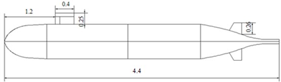
The geometrical size of the underwater vehicle was shown in Fig. 1. The length of the command platform was 0.4 m and the height was 0.25 m. The underwater vehicle tail was designed to be cross-shaped tail wing. The total length of the underwater vehicle was 4.4 m. The distance between the command platform and the vehicle’ head was 1.2 m. The highest point of the cross-shaped tail wing was 0.26 m far from the underwater vehicle. Taking the height direction of the underwater vehicle as $x$ axis and the center line from the head to the tail as $y$ axis, thus a reference coordinate system was built.

Fig. 1Geometrical size of the underwater vehicle

3.1. Mesh generation

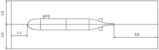
The structured and unstructured meshes were applied, and a good computational accuracy was obtained. The total mesh number was 1,366,336, as shown in Fig. 2. In order to make the numerical computation results more accurate, the computational domain of the underwater vehicle should be as large as possible. In this paper, the computational domain size was shown in Fig. 3. In $x$ direction, the distance between the center line of the vehicle and the computational domain boundary was 6 m. In $y$ direction, the distance between the head of the vehicle and the computational domain boundary was 3.5 m, and the distance between the tail and the computational domain boundary was 8.6 m. To accurately describe the flow and capture the flow information which was close to the wall, the computational velocity was adopted as 5.93 knots (3.05039 m/s), and $R_{e} =$ 1.3248×10⁷. The computational steps were as follows. Firstly, the stream flow velocity was given to carry out steady computation, and then the simulation accuracy was verified after its full convergence. When we obtained a satisfying accuracy, the steady solution would be treated as the initial value of the unsteady computation. The time step of the unsteady computation was taken as 0.00005 s to capture high-frequency noise.

Fig. 2Surface meshes of SUBOFF underwater vehicle model

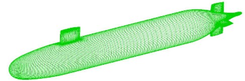
Fig. 3Computational area of the underwater vehicle

3.2. Simulation result and analysis of the flow field for the underwater vehicle

Through the above analysis and computation, the velocity distribution of the surface for the underwater vehicle could be obtained as shown in Fig. 4. It could be seen that the flow velocity was relatively large at the head and tail. In order to further research the influence of the velocity distribution on the near field, the power spectrum density of the head, the middle part and the tail were extracted, respectively, as shown in Fig. 5.

Fig. 4Surface velocity distribution of the underwater vehicle

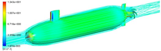
Fig. 5Power spectrum density of the head, middle part and the tail for the underwater vehicle

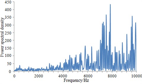
a) Power spectrum density near the head of the underwater vehicle

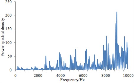
b) Power spectrum density near the middle part of the underwater vehicle

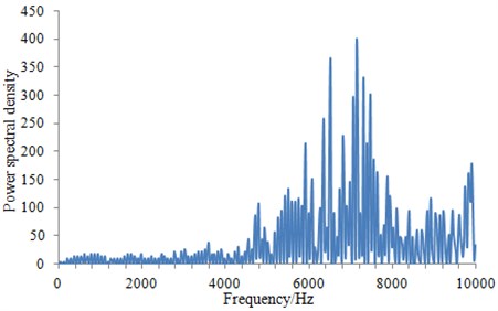
c) Power spectrum density near the tail of the underwater vehicle

It can be seen from Fig. 5 that power spectrum density at the head and the tail was much larger than that at the middle part. This was mainly due to that there were some appendages at the two places of the underwater vehicle, such as command platform and the cross-shaped tail wing. These appendages had a serious influence on the distribution of the flow field around the underwater vehicle. When power spectrum density was large, the underwater vehicle would cause larger radiation noise. At present, there were many researches on command platform of the underwater vehicle. A lot of work has been done for the shape optimization of command platform. As a result, command platform shape and location in this paper were close to the ideal state, so that it had no much significance to further optimize noise. Therefore, this paper tried to optimize the tail to reduce the radiation noise from the vehicle.

The fluid meshes in Fig. 1 were taken as the basis, and a boundary element model was built, as shown in Fig. 6. The boundary element model applied a quadrilateral shell element, and it was made of 2650 elements and 2147 nodes.

The surface velocity distribution of the underwater vehicle computed in Fig. 4 and the boundary element model in Fig. 6 were then imported into Virtual.lab software. Then, the surface velocity of the underwater vehicle was mapped to the boundary element model, and the acoustic vibration coupling was computed. As a result, sound field distribution of the underwater vehicle surface was obtained, as shown in Fig. 7. It can be seen from Fig. 7 that sound pressure of the head and the tail were relatively large, and the distribution of sound field was relatively disordered.

Fig. 6Boundary element model of the underwater vehicle

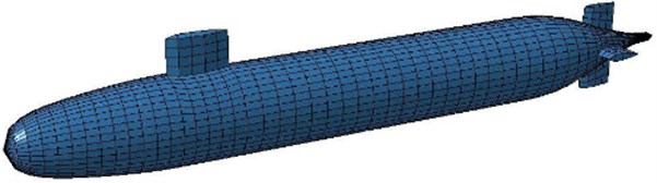
Fig. 7Contour of sound field distribution for the underwater vehicle

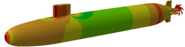
Fig. 8Sound pressure level at the observation point

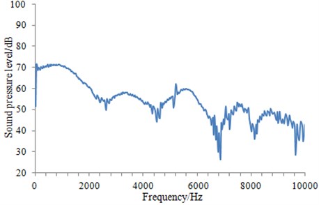
When sound field of the underwater vehicle was computed, an observation point was set up in the front of the vehicle to monitor the radiation noise in near field. Sound pressure level of the observation point was extracted, as shown in Fig. 8.

It can be seen from Fig. 8 that the radiation noise of the vehicle had a decreasing trend in the whole frequency range. And at some points, there would be a big fluctuation. At low frequency, the radiation noise of the vehicle was larger, because this radiation noise included not only flow noise, but also mechanical noise. In addition, mechanical noise was larger than flow noise. At high frequency, the mechanical noise of the vehicle was small and could be neglected, so noise can be considered as flow noise.

3.3. Analysis and verification of the flow noise for the underwater vehicle

The numerical computation of the radiation noise for the underwater vehicle was a very complicated process. Therefore, it was necessary to verify the accuracy of the computational results through experiments.

In this paper, the radiation noise of the underwater vehicle was tested in the shallow sea, as shown in Fig. 9. There was a buoy on the water surface, which provided guidance for the safety driving of the underwater vehicle. A floating block and a sinking block were placed under water to arrange a sensor array system in their middle. In addition, in order to ensure that sensor array system would not shake because of external reasons, a balance block was mounted between the sensor array system and the sinking block. The cable was connected to the laboratory, and then the test was conducted. The experimental conditions were consistent with the numerical simulation process to the greatest extent, and test time was 10 s. The experiment was conducted for three times. The average value was taken as the final experimental value and compared with that of the numerical simulation, as shown in Fig. 10.

Fig. 9Diagram of the radiation noise experiment of the underwater vehicle

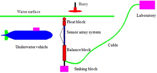
Fig. 10Comparison of the radiation noise between experiment and simulation

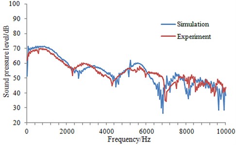
It can be seen from Fig. 10 that the computational results were consistent with those of the experimental in overall change trend. In addition, the size was also similar. At some frequency points, the computational results had a trough, and the experimental value was also similar at the adjacent frequency. Therefore, it indicated that the computation model in this paper was reliable and can be used for the subsequent analysis.

4. Changing tail wing of the underwater vehicle

The X-shaped tail wing was chosen for the underwater vehicle, with the underwater vehicle having the same sizes as the previous. Furthermore, the section of NACA0020 type was also selected for the tail wings, and the tail wing was still 0.26 m away from the underwater vehicle. Moreover, the tail wing arrangement was changed from the traditional cross-shaped type into the symmetrical X-type which was 45° with the transverse and longitudinal sections of the underwater vehicle, as shown in Fig. 11. The mesh size was equal to that of the cross-shaped, so as to make a better comparison between the computational results.

Fig. 11Two different kinds of tail wings

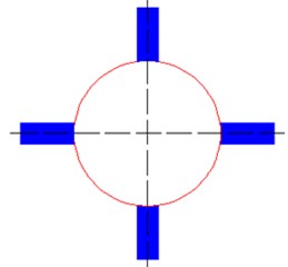
a) Cross-shaped tail wing

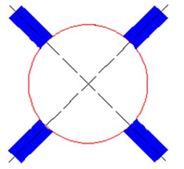
b) X-shaped tail wing

4.1. Computational results and analysis of the flow field for the underwater vehicle with two kinds of tail wings

The velocity distribution on the symmetry plane of the underwater vehicle with cross-shaped tail wing was shown in Fig. 12(a), while that of the X-shaped in Fig. 12(b).

Fig. 12Comparison of velocity distributions on symmetry plane of the underwater vehicle with two kinds of tail wings

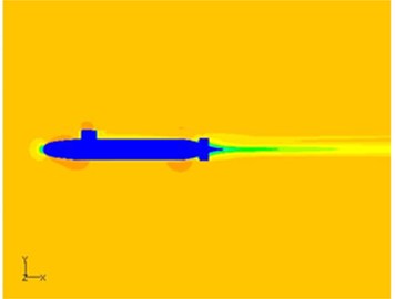
a) Velocity distribution on symmetry plane of the underwater vehicle with cross-shaped tail wing

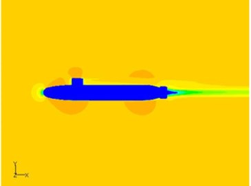
b) Velocity distribution on symmetry plane of the underwater vehicle with X-shaped tail wing

It can be seen from Fig. 12(a) and Fig. 12(b) that the major difference was that the area with high speed flow at the front of the tail wings and command platform for the X-shaped was larger than that of the cross-shaped. The reason was that the blocking effect of the X-shaped tail wing got weaker than that of the traditional cross-shaped, thus the flow accelerated area became bigger.

4.2. Computational results and analysis of the flow noise for the underwater vehicle with two kinds of tail wings

The sound pressure level at the observation point of the underwater vehicle with two kinds of tail wings was compared, as shown in Fig. 13.

Fig. 13Comparison of sound pressure levels at observation point of the underwater vehicle with two kinds of tail wings

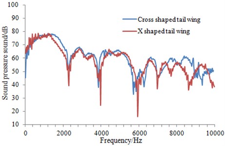
It can be seen from Fig. 13 that the change trend of the radiation noise obtained from the underwater vehicle with two kinds of tail wings was of little difference. The radiation noise of the underwater vehicle with cross-shaped tail wing was relatively larger. However, the radiation noise of the underwater vehicle with X-shaped tail wing was significantly smaller at some frequency point. This was mainly due to that X-shaped tail wing changed the overall layout of the rear structure, making the flow field distribution around the underwater vehicle change.

In order to further observe the influence that X-shaped tail wing had on the radiation noise of the underwater vehicle in the whole dimensions, the radiation noise sound pressure level from head to tail of the underwater vehicle was calculated, as shown in Fig. 14.

Fig. 14Total sound level comparison of the radiation noise at each point along the length of the underwater vehicle with two kinds of tail wings

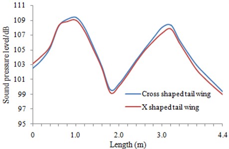
As can be seen from Fig. 14, for the vehicle with X-shaped tail wing, there was a certain improvement for its radiation noise, but the change was not great. So it was necessary to conduct further research on the influence that X-shaped tail wing had on the radiation noise of the underwater vehicle.

5. The optimization of the radiation noise for the underwater vehicle with X-shaped tail wing

According to the above analysis, it can be found that the radiation noise of the underwater vehicle with X-shaped tail wing was improved to some extent, but the improvement was not very obvious. Therefore, this paper attempted to research the position and local shape of X-shaped tail wing in order to further optimize the radiation noise.

5.1. Changing the position

In the above analysis, X-shaped tail wing was in A position of the underwater vehicle, as shown in Fig. 15. This paper attempted to move it to B position and remained the size and shape of X-shaped tail wing unchanged. And then, the radiation noise at observation point was computed and compared with the original results, as shown in Fig. 16.

Fig. 15Position of X-shaped tail wing for the underwater vehicle

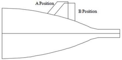
Fig. 16Comparison of the radiation noise between different positions for X-shaped tail wing

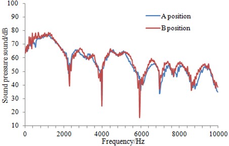
It can be seen from Fig. 16 that the radiation noise of the underwater vehicle was improved to some extent when X shaped tail wing was placed in B position. Especially at high frequency, this effect was more obvious. As for the optimal position of X-shaped tail wing, it was unable to be accurately obtained by using the existing optimization algorithms. The optimization algorithm was based on a certain mathematical model, which simplified or neglected the original boundary conditions, and it failed to reflect the most real situation. Currently, position of X-shaped tail wing’s can be only obtained based on the numerical simulation. For this situation, this paper computed the radiation noise of the underwater vehicle with dozens of different positions tail wing. Finally, it was found that X-shaped tail wing at B position was relatively optimal. Therefore, the subsequent research would be conducted based on B position.

5.2. Fillet filling

The mentioned X shaped tail wing was without fillet filling at the position where was connected with the underwater vehicle, so the transition was relatively sharp and not smooth. Therefore, based on B position, the fillet filling was carried out on the connection between X shaped tail wing and the underwater vehicle, as shown in Fig. 17. Similar to the position selection of X shaped tail wing, the optimal fillet filling angle can only be obtained by means of a lot of simulation results. Finally, the radiation noise of the underwater vehicle with fillet filling tail wing was compared with that of the underwater vehicle without fillet filling, as shown in Fig. 18.

Fig. 17X-shaped tail wing with fillet filling

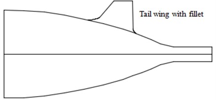
Fig. 18Influence on the radiation noise of the underwater vehicle by fillet filling

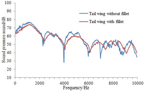
As can be seen from Fig. 18, the radiation noise of the underwater vehicle with fillet filling had not changed obviously in the overall trend, but the value was obviously changed. And the radiation noise of the underwater vehicle was relatively smooth in the whole frequency band. This was mainly for the reason that the fluid of the tail can more easily pass X-shaped tail wing after fillet filling.

6. Conclusions

In this paper, Reynolds Average Navier-Stokes equation (RANS) with turbulence model and FW-H acoustic model were adopted to compute the flow field and the flow noise of the underwater vehicle. It could be obtained from the computational results that the tail wing had a great influence on the flow noise of the underwater vehicle. Consequently, to reduce resistance and noise, the traditional cross-shaped tail wing was changed into the symmetrically-arranged X-shaped which was 45° with the transverse and longitudinal sections of the underwater vehicle. After that, the numerical simulation on the resistance and flow noise of the improved X-shaped tail wing arrangement was conducted, which indicated that the blocking effect of the flow field by the improved X-shaped was weaker than that by the traditional cross-shaped. In addition, the flow noise of X-shaped tail wing was improved at a certain extent. However, the improvement was not very obvious. Therefore, this paper attempted to research the position and local shape of X-shaped tail wing in order to further optimize the radiation noise.

References

Iglesias O., Lastras G., Canals M., et al. The BIG’95 submarine landslide-generated tsunami: a numerical simulation. The Journal of Geology, Vol. 120, Issue 1, 2012, p. 31-48.

Search CrossRef
Font R., García-Peláez J. On an underwater vehicle hovering system based on blowing and venting of ballast tanks. Ocean Engineering, Vol. 72, 2013, p. 441-447.

Search CrossRef
Cremonesi M., Frangi A., Perego U. A Lagrangian finite element approach for the simulation of water-waves induced by landslides. Computers and Structures, Vol. 89, Issue 11, 2011, p. 1086-1093.

Search CrossRef
Chase N., Michael T., Carrica P. M. Overset simulation of an underwater vehicle and propeller in towed, self-propelled and maneuvering conditions. International Shipbuilding Progress, Vol. 60, Issue 1, 2013, p. 171-205.

Search CrossRef
Zhang N., Yang R. Y., Shen C. H. Numerical towing tank and CFD simulation for the underwater vehicle powering performance. Journal of Ship Mechanics, Vol. 15, Issues 1-2, 2011, p. 17-24.

Search CrossRef
Atkins D. J. Computational hydrodynamics for the underwater vehicle – recent development. International Symposium on Naval Submarine, Vol. 5, 1996.

Search CrossRef
Wang M., Lele S. K., Moin P. Sound radiation during local laminar breakdown in a low-Mach-number boundary layer. Journal of Fluid Mechanics, Vol. 319, 1996, p. 197-218.

Search CrossRef
Piomelli U., Streett C. L., Sarkar S. On the computation of sound by large-eddy simulations. Journal of Engineering Mathematics, Vol. 32, Issues 2-3, 1997, p. 217-236.

Search CrossRef
Bastin F., Lafon P., Candel S. Computation of jet mixing noise due to coherent structures: the plane jet case. Journal of Fluid Mechanics, Vol. 335, 1997, p. 261-304.

Search CrossRef
Lighthill M. J. On sound generated aerodynamically. I. General theory. Proceedings of the Royal Society of London. Series A. Mathematical and Physical Sciences, Vol. 211, Issue 1107, 1952, p. 564-587.

Search CrossRef
Arakeri V. H., Satyanarayana S. G., Mani K., et al. Studies on scaling of flow noise received at the stagnation point of an axisymmetric body. Journal of Sound and Vibration, Vol. 146, Issue 3, 1991, p. 449-462.

Search CrossRef
Launder B. E., Spalding D. B. The numerical computation of turbulent flows. Computer Methods in Applied Mechanics and Engineering, Vol. 3, Issue 2, 1974, p. 269-289.

Search CrossRef
Xu S. R. Noise reduction of shell and tail of command room for the underwater vehicle. The Eighth National Colloquium of Ship Underwater Noise, 2001.

Search CrossRef
Zhang H. X., Fan X. B., Sun H. X. Test Report of the Underwater Vehicle Model Flow Noise, Technical Report. China Defense Science and Technology Report. 2007.

Search CrossRef

About this article

Received

27 August 2014

Accepted

16 July 2015

Published

15 August 2015

SUBJECTS

Flow induced structural vibrations

Keywords

computational fluid dynamics

flow field

flow noise

tail wing type

blocking effect

This is an open access article distributed under the Creative Commons Attribution License, which permits unrestricted use, distribution, and reproduction in any medium, provided the original work is properly cited.