Research on the characteristics of aerodynamic noise for wind turbines by considering non-compact Green’s boundary conditions

Zhang, Wei

Journal of Vibroengineering

Browse Journal

Submit article

Published: 31 March 2015

Check for updates

Research on the characteristics of aerodynamic noise for wind turbines by considering non-compact Green’s boundary conditions

Wei Zhang¹

¹Mechanical Engineering Institute, Zhejiang Institute of Mechanical and Electrical Engineering, Zhejiang, Hangzhou, 310053, China

Cite the article Download PDF

Downloads 1319

Abstract

The aerodynamic noise of wind turbines mainly concentrate in low-frequency range, with small corresponding air absorption coefficient. The noise is mainly caused by the friction between the rotating wind turbine blades and the air, and is greatly related to the parameters such as the surface and angle of the wind turbine blades. In this paper, the flow field surrounding the symmetrical airfoils in Large Eddy Simulation (LES) model was computed by finite element method; the sound field of the aerodynamic noise was simulated by Lighthill acoustic analogy method; aerodynamic characteristics and sound pressure levels at the monitoring points were compared with the experiment results, which showed that they were almost identical. To eliminate the influences of boundary conditions, actual situations use High Reynolds number, low Mach number, frequency domain boundary stationary FW-H equation, and the influence of non-compact Green’s boundary was considered to compare the value results of sound pressure acquired from FFT conversion and the analytical results, which showed that the two results were identical. This research has special value and can provide references for designing the airfoil profiles of wind turbines in future.

1. Introduction

Wind power doesn’t need to burn any fuel or emit any harmful gas, so it is known as the cleanest and inexhaustible renewable energy. The noise from the wind turbine sets during their operation affects the residents in certain range. For this reason, aerodynamic noise from wind turbine has become a highlighted issue in environmental noise research and prevention analysis.

Numerous scholars [1-3] have carried out abundant experiments and theoretical researches about aerodynamic noise. Lighthill [4, 5] proved that aerodynamic noise problem could be an analogy of acoustics, which formed famous Lighthill acoustic analogy theory. Curle [6] solved Aeolian noise of static objects in turbulent flow and the noise induced by eddy-shedding of flow around a circular cylinder etc. Ffowcs Williams and Hawings [7] derived famous FW-H equation. Rotor noise is generally calculated on the basis of FW-H equation. Han [8] carried out transonic speed two-dimensional experiment on airfoil profile in a wind tunnel, and obtained correct chord-wise pressure distribution for this airfoil profile; he also compared this with the experiment result in large wind tunnels, thus exploring the interference of tunnel wall on the flow characteristics of the airfoil profile and corrected it.

The above-mentioned researches on the airfoil profile noise of wind turbines mainly focus on airfoils with symmetrical profiles such as NACA0012 and NACA0018 etc. The experiment conditions for the model include low Reynolds number, high Mach number and large stalling attack angle. However, the actual working conditions for wind turbine are high Reynolds number and low Mach number; therefore, it is necessary to research this. Considering non-compact Green’s boundary which is often ignored in wind turbine noise simulation, the airfoil profile of the wind turbine is further optimized and is compared with the experiment results. This research has special value and can provide references for designing the airfoil profile of wind turbines in future.

2. Theories

Firstly, pulsating pressure around the airfoil profile was calculated by large eddy simulation; then the sound field around the airfoil profile was calculated by means of Lighthill acoustic analogy method. When the pressure field was stable, the sound field information, and sound pressure spectrogram at the monitoring points as well as the eddy fields at the front-stage and back-stage impellers were extracted to analyze the distribution and change of strength of the eddy fields on the impellers under different attack angles. To verify the reliability of this simulation method, the results were compared with the experiment values in Reference [9], which showed that they were identical. For non-compact structures, the aerodynamic noise excited by unsteady flow will reflect and scatter on the structure wall while radiating to the space, which will result in the situation that the actual sound field of the aerodynamic noise is obviously different from the radiated sound field under free space. Therefore, the influence of non-compact boundary [10-12] on aerodynamic noise should be considered in simulation calculation.

2.1. Control equation of large eddy numerical simulation

Large eddy simulation method can effectively observe the transient characteristics of the flow field. Its basic thought is to filter N-S equation in a physical space to directly calculate large-scale pulsation, to simulate small-scale turbulent motion by sub-grid scale model, and to simulate filter function by large eddy simulation to deal with N-S equation and continuity equation under transient state:

1

\frac{\partial}{\partial t} (ρ {\bar{u}}_{i}) + \frac{\partial}{\partial x_{i}} (ρ \bar{u_{i} u_{j}}) = - \frac{\partial \bar{P}}{\partial x_{i}} + \frac{\partial}{\partial x_{i}} (μ \frac{\partial {\bar{u}}_{i}}{\partial x_{j}}) + \frac{\partial τ_{i j}}{\partial x_{j}},

2

\frac{\partial ρ}{\partial t} + \frac{\partial}{\partial x_{j}} (ρ {\bar{u}}_{j}) = 0 .

Turbulent flow velocity is the sum of low-pass pulsation $u_{i}$ and residual pulsation $u_{i}^{″}$ . Similarly, the pressure is the sum of low-pass pressure $p$ and residual pressure $p^{″}$ . As the Mach number on the cross sections of airfoil profiles of the wind turbine blades is smaller than 0.3, therefore, the air can be considered as incompressible fluid. N-S equation can be filtered to acquire the following equation:

3

\frac{\partial {\bar{u}}_{i}}{\partial t} + \frac{\partial {\bar{u}}_{i} {\bar{u}}_{j}}{\partial x_{j}} = - \frac{1}{ρ} \frac{\partial \bar{p}}{\partial x_{i}} + ν \frac{\partial^{2} {\bar{u}}_{i}}{\partial x_{j} \partial x_{j}} + \frac{\partial ({\bar{u}}_{i} {\bar{u}}_{j} - \bar{u_{i} u_{j}})}{\partial x_{j}},

4

\frac{\partial {\bar{u}}_{i}}{\partial x_{j}} = 0,

5

{\bar{τ}}_{i j} = ({\bar{u}}_{i} {\bar{u}}_{j} - \bar{u_{i} u_{j}}) = 2 {(C_{S} ∆)}^{2} {\bar{S}}_{i j} (2 {\bar{S}}_{i j} {\bar{S}}_{i j}) 1 / 2 - \frac{1}{3} {\bar{τ}}_{k k} δ_{i j} .

In the aforesaid equation, $i$ , $j$ and $k$ are direction variables, and $ρ$ is fluid density, while ${\bar{u}}_{i}$ and ${\bar{u}}_{j}$ are the velocity components after filtering. In addition, $ν$ is viscosity coefficient of the turbulent flow, and $- τ$ is referred to as sub-grid stress, and $Δ$ is filter scale. This sub-grid stress model refers to as Smagorinsky mode.

2.2. Lighthill acoustic analogy theory

Lighthill proposed the basic theory of aero-acoustics as follows:

6

\frac{\partial^{2} (ρ - ρ_{0})}{\partial t^{2}} - \frac{\partial}{\partial x_{i}} (c_{0}^{2} \frac{\partial (ρ - ρ_{0})}{\partial x_{i}}) = \frac{\partial^{2} T_{i j}}{\partial x_{i} \partial x_{j}} .

In the equation: $ρ_{0}$ is ambient density which is a constant. $(ρ - ρ_{0})$ are the fluctuation variables of the fluid density. $c_{0}$ is sound velocity. $T_{i j}$ is Lighthill stress tensor. Eq. (6) can be derived by Green’s function to acquire the following fractions:

7

ρ - ρ_{0} = \frac{1}{C_{0}^{2}} \int_{- T}^{T} \int_{υ (τ)} \frac{\partial^{2} G}{\partial y_{i} y_{j}} T_{i j} d y d τ + \frac{1}{C_{0}^{2}} \int_{- T}^{T} \int_{s (τ)} \frac{\partial G}{\partial y_{i}} f_{i} d s (y)

+ \frac{1}{C_{0}^{2}} \int_{- T}^{T} \int_{s (τ)} ρ V_{n} \frac{D_{0} G}{D_{τ}} d s (y) d τ .

The first term on the right of the fraction represents the quadripoles (stress inside the fluid) of the fluid flowing, the second term represents the dipoles (dual pressures applied on the solid surface by the fluid) of the fluid flowing, the third term represents monopole of the volume displacement caused by the solid boundary.

2.3. Non-compact Green’s function

To simplify the analysis, FW-H equation of the frequency domain under the condition of high Reynolds number, low Mach number and static boundary taken into consideration in this paper:

8

C_{0}^{2} P_{a} (x, ω) = - \int_{Ω} \frac{T_{i j} \partial^{2} G (x, y, ω)}{\partial y_{i} \partial y_{j}} d y - \int_{S} \frac{P \partial G (x, y, ω)}{\partial n (y)} d s (y) .

In the equation, $x$ and $y$ represent the observation points and point source positions respectively, $Ω$ is sound source area, $S$ is boundary, $P$ indicates the force applied on the fluid by the solid surface in unit area, $P_{a}$ indicates acoustic density pulsation, $ω$ indicates circular frequency.

$G (x, y, ω)$ is the Green’s function of the frequency domain. It meets the follows:

9

(\frac{ω^{2}}{C_{0}^{2}} + \nabla_{y}^{2}) G (x, y, ω) = - δ (x - y) .

For non-compact structures with acoustic hard boundary, Green’s function $G (x, y, ω)$ should meet the follows:

10

\frac{\partial G (x, y, ω)}{\partial n (y)} = 0 .

In Eq. (10), $n$ is the unit normal vector of boundary $S$ , its positive direction directs towards sound source area from the boundary. Therefore, Eq. (8) can be simplified as:

11

C_{0}^{2} P_{a} (x, ω) = - \int_{Ω} \frac{T_{i j} \partial^{2} G (x, y, ω)}{\partial y_{i} \partial y_{j}} d y .

3. Finite element numerical simulations

3.1. Acoustic grid model and arrangement of monitoring point for airfoil

Discrete noise of the wind turbine is caused by the interaction between the periodically rotating impellers and the surrounding barriers. The flow and noise of the internal flow field of the two-stage impellers of the wind turbine are the most complicated. See Fig. 1 for the grid model of airfoil profile of the wind turbine. See Fig. 2 for the control for horizontal monitoring points. The main monitoring points were arranged at the positions near the inlet and outlet of the two-stage impellers and inside the two-stage impellers. Airfoil chord length $c =$ 60 mm, the computational domain was a circle with the diameter of 3 m.

Fig. 1Chart of airfoil profile grids

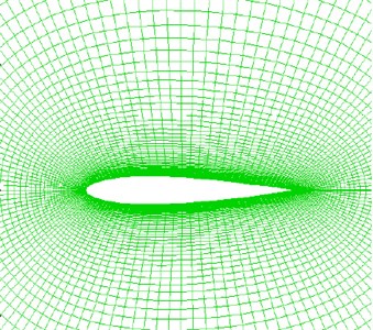
Fig. 2Arrangement of the boundary of sound field grids

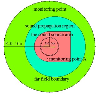
Fig. 3Control or noise monitoring

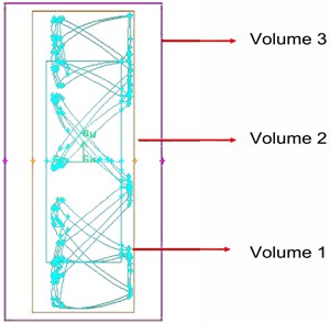
Fig. 4Distribution of airfoil grids and boundary space

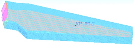
Fig. 5Lift coefficients under different attack angles

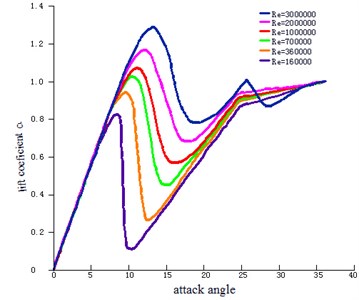
The circle included two parts of internal domain and external domain. Structured grids were constructed in ICEM. The boundary layer thickness of the first layer outside the airfoil was 0.03 mm, and the total grid number was 1.5 million. The external boundary was set as the pressure far field, and the airfoil was set as a non-slipping wall. See Fig. 3 for the control for longitudinal monitoring along the airfoil. Fig. 4 indicates the relationship between the space grids of the airfoil profile of the wind turbine and the boundary. Fig. 5 provides the curve of lift coefficient change of the airfoil profile of the wind turbine under different attack angles.

Fig. 5 indicates that under high Reynolds number condition, the airfoil profile of the wind turbine can obtain high lift coefficient and damping ratio. Further verification is required to see whether the sound field characteristics under low Reynolds number comply with this conclusion.

3.2. Noise analysis of the airfoil

To simulate the flow field and sound field around the symmetrical airfoil profile, the computation Reynolds number $R e =$ 1.6×10⁵ and inflow velocity $υ =$ 24 m/s were taken. When the pressure field was stable, the sound pressure level at monitoring point A was extracted, as shown in Fig. 6. It shows that the sound pressure level reduces as the frequency increases and the sound pressure level gradually increases as the attack angle increases. To verify the correctness of this numerical simulation, the test results at the monitoring point were extracted to compare with it. The sound pressure level spectrograms under the attack angles of $α =$ 0°, $α =$ 3°, $α =$ 6° and $α =$ 9° were extracted, as shown in Fig. 7.

Fig. 6Sound pressure spectrogram at monitoring points

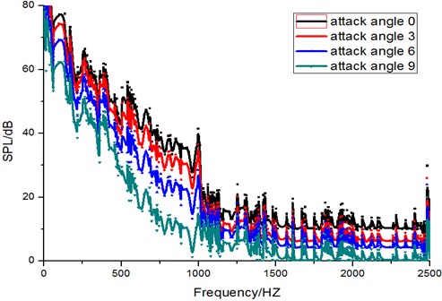
Fig. 7Sound pressure spectrogram at monitoring points

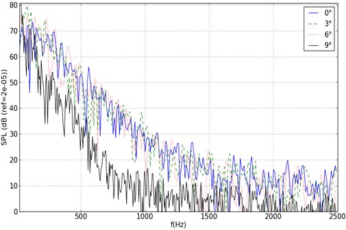
The numerical simulation results in Fig. 6 and the test results in Fig. 7 were compared, which showed that they were identical. This verifies the effectiveness of this numerical simulation. When the attack angle is 9°, the difference between them is the maximum. This is because with the increase of the attack angle, serious separated flow occurs at the trailing edge of the impeller, which results in complicated flow field near the trailing edge of the airfoil, thus leading to the huge error between the numerical simulation and the test. However, its tendency shows that when the attack angle is 9°, the sound pressure level also tends to be stable.

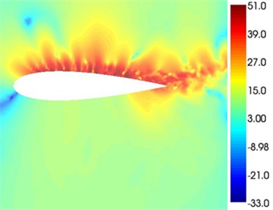
Fig. 8-Fig. 11 indicates the chart of the sound pressures around the airfoil under four attack angles when the frequency is 2000 Hz. When the attack angle is 0°, the chart of the sound pressures above and under the airfoil are symmetrical, and the main sound sources are located in the trailing edge and the wake flow. As the attack angles increases, the sound source area located at the trailing edge of the airfoil approaches towards the leading edge of the airfoil on the sucking surface. When the attack angle is 12°, the red sound source area basically covers the sucking surface of the airfoil. The reason for this is that with the increase of the attack angle, the position where the upper eddy shedding occurs on the airfoil suction surface moves towards the leading edge, thus making the position where the separated flow noise occur move towards the leading edge.

Fig. 8α= 0° chart of the sound pressure

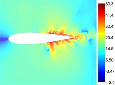
Fig. 9α= 6° chart of the sound pressure

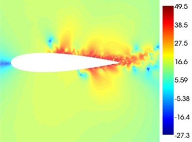
Fig. 10α= 9° chart of the sound pressure

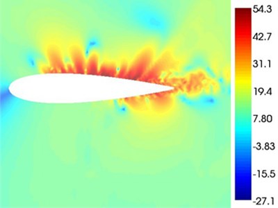
Fig. 11α= 12° chart of the sound pressure

3.3. Eddy field distribution of the airfoil

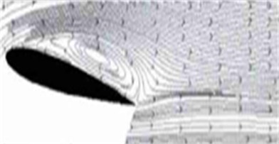
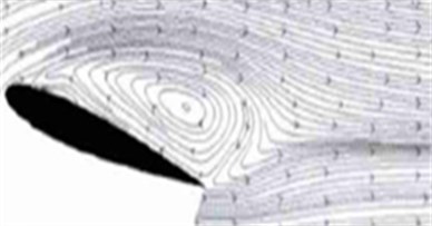
Wu Yun [9] researched the flow characteristics of NACA0012 airfoil at $R e =$ 8200 by means of hydrogen bubble flow visualization in the sink and PIV velocity measurement test. The change of the incidence angle (0-16°) of the airfoil profile was realized by adjusting the angle location hole on the end plate. The hydrogen bubble flow coordinates were built by means of Cartesian left hand coordinate system to indicate $x$ - $y$ side-looking plane and $x$ - $z$ overlooking plane by hydrogen bubble flow visualization. Velocity field measurement was carried out for the $x$ - $y$ side-looking plane by means of time-continuous two-dimensional PIV system, with the emphasis on the change the structure of flow around airfoil profile as the incidence angle changes. The flow conditions of NACA0012 airfoil under numerical simulation were divided into 3 ranges: small incidence angle (0-3°), medium incidence angle (6-8°) and large incidence angle (10-15°). This was compared with the experiment result from reference [9] in order to verify whether the simulation result was correct. As shown in Fig. 12, in the range of small incidence angle, the flow attaches to the airfoil surface, or forms small backflows near the trailing edge of the airfoil profile or near the wake area. At this time, the flow in most area of the airfoil profile is in attaching status, and the position turned up by the eddy is located at the rear of the airfoil profile and in the wake; moreover, with the increase of the incidence angle, the separation point gradually moves towards the front of the airfoil profile, which is consistent with the experiment results in Fig. 13. As shown in Fig. 14, in the range of medium incidence angle, as the adverse pressure gradient on the upper surface of the airfoil profile strengthens, the shear layer separation point moves towards the upstream to the front of the airfoil profile to make the upper surface of the airfoil profile form separation eddy, the eddy sheds from the separation shear layer, with its scale gradually increasing during the process of convection downstream. This is consistent with the experiment result in Fig. 15. As shown in Fig. 16, in the range of large incidence angle, the adverse pressure gradient on the upper surface further strengthens，the eddy on the upper surface of the airfoil profile has moved to the front of the airfoil profile, and the flow separates at the position near the front of the airfoil profile. At this time, forced by adverse pressure gradient, the fluid cannot attach to the surface. The separated free shear layer keeps away from the surface of the airfoil profile and develops towards the downstream direction and no longer attaches to the upper surface of the airfoil profile. This is consistent with the experiment result in Fig. 17. Comparison between experiment and numerical simulation indicates the follows: under low Reynolds number, local eddy pairing phenomenon can be observed in the structure of flow around NACA0012 airfoil profile and its evolution under small and medium incidence angle. In large incidence angle range, the time-averaged separation point moves to the front of the airfoil profile. At this time, the airfoil will be in stall conditions, which is identical with the actual working conditions of wind turbines. Meanwhile, it also verifies the reliability of numerical simulation.

Fig. 12α= 0° chart of eddy field for simulation

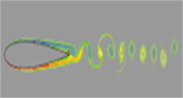
Fig. 13α= 0° chart of eddy field for experiment

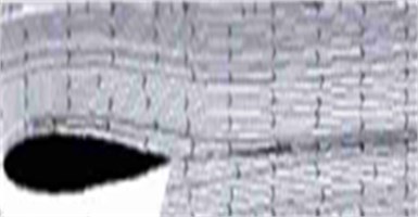
Fig. 14α= 8° chart of eddy field for simulation

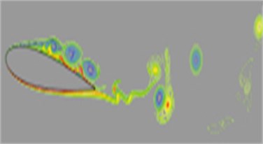
Fig. 15α= 8° chart of eddy field for experiment

According to the aforesaid eddy diagrams, the eddy strength on the sucking surface of the blades is larger than that under the pressure surface. The positions with the maximum eddy strengths centralize at the blade top, leading edge and trailing edge of each surface of the blades. In the middle of the blades, the eddy system gradually dissipates along the blade from top to down. The eddy strengths on the pressure surface and sucking surface of the blades of the back-stage impeller are obviously larger than that on the pressure surface and sucking surface of the blades of the front-stage impeller. This indicates that the airflow in the passage of the back-stage impeller is more turbulent than that in the passage of front-stage impeller, with comparatively large flow field pressure gradient. The airflow in the inter-stage flow field bears the combined actions of the two-stage impellers, which results in serious turbulent flow in the flow field, thus enlarging the eddy strength in the passage of the back-stage impeller.

Fig. 16α= 15° chart of eddy field for simulation

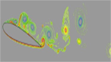
Fig. 17α= 15° chart of eddy field for experiment

3.4. Influence of non-compact Green’s boundary

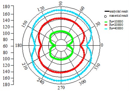
To make the sound pressure results in the near field and far field of the monitoring points more visual, the directivity patterns are extracted, which are as shown in Fig. 18 and Fig. 19. Fig. 20 is the directivity pattern of the far-field sound pressure of the airfoil by considering non-compact Green’s boundary condition. Non-compact Green’s function is divided into two parts of scattering term and incidence term by numerical analysis method. Quantitative analysis can be carried out on the influence of wall scattering on the sound field. The calculation example results indicate that with the increase of wave numbers, the scattering influence of non-compact acoustic boundary becomes increasingly obvious. On the other hand, it shows that the numerical results are identical with the analysis results.

Fig. 18Directivity pattern of near-field sound pressure

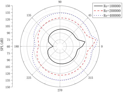
Fig. 19Directivity pattern of far-field sound pressure

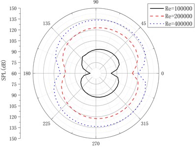
Fig. 20Directivity pattern of far-field sound pressure under non-compact Green’s boundary condition

4. Conclusions

1) According to the distribution of sound power of aerodynamic noise, the area where the two-stage impellers of the wind turbine with comparatively where high wind turbine noise exists, so this area should be deemed as a key area for researching wind turbine noise. Several monitoring points are set at the internal flow field of the two-stage impellers of the wind turbine. Inter-stage flow field and the areas in front of and behind the impellers, so as to carry out researches on the inter-stage flow field from the perspectives of pressure and eddy distribution.

2) The pressure gradients at the positions such ass boundary layer, blade surface and blade top etc. are large. Meanwhile, the eddy at these positions is also intense. The eddy strength value changes with the change of pressure gradient. The eddy strength value on the blade top is higher than that on the two sides of the blade, and the eddy strength value on the blade sucking surface is higher than that on the blade pressure surface.

3) The eddy strength in the area surrounding the blades is comparatively large. In the flow field, the eddy at the positions without contacting the solid walls is small. This shows that the positions where eddy occurs are those surrounding the internal solid wall of the flow field, i.e., the eddy is caused by mutual effects between the air and the solid wall. In the same impeller, the eddy strength on the front detecting surface is the maximum. The eddy strength reduces as the airflow flows in both the front-stage and the back-stage impellers.

4) Based on boundary element thought, the existence of non-compact Green’s boundary makes the values of Green’s function fluctuate in different directions. With the increase of the fluctuation, the scattering influence of non-compact boundary becomes larger and larger.

References

Jones A. D., Hu F. Q. An investigation of spectral collocation boundary element method for the computation of exact Green’s functions in acoustic analogy. 12th AIAA/CEAS Aeroacoustics Conference, Cambridge, Massachusetts, 2006.

Search CrossRef
Golerfelt X., Perot F., Bailly C., June D. Flow-induced cylinder noise formulated as diffraction problem for low. CEAS Aeroacoustics Conference, Cambriage, Massachusetts, 2007.

Search CrossRef
Takaishi T., Miyazawa M., Kato C. Computational method of evaluating noncompact sound based on vortex sound theory. The Journal of Acoustical Society of America, Vol. 121, 2007, p. 1353-1361.

Search CrossRef
Lighthill M. J. On sound generated aerodynamically. I. General theory. Proceedings of Royal Society. Vol. A211, 1954, p. 1-32

Search CrossRef
Lighthill M. J. On sound generated aerodynamically. II. Turbulence as a theory of sound. Proceedings of Royal Society, Vol. A221, 1954, p. 1-32

Search CrossRef
Curle N. The influence of solid boundaries upon aerodynamic sound. Proceedings of Royal Society, Vol. A231, 1955, p. 504-514.

Search CrossRef
Ffowcs Williams J. E., Hawkings D. L. Sound generatwd by turbulence and surfaces in arbitrary motion. Philosophical Transactions of the Proceedings of Royal Society, Vol. A264, 1969, p. 321-342.

Search CrossRef
Han B. Z., Huang Y. Y., Zhang Q. W., Cheng P. R. An experiment of pressure measurement for NACA0012 airfoil in a transonic wind tunnel. Journal of Nanjing Aeronautical Institue, Vol. 2, Issue 6, 1987, p. 92-102.

Search CrossRef
Wu Y., Wang J. J., Li T. Experimental investigation on low Reynolds number behavior of NACA0012 airfoil. Journal of Experiments in Fluid Mechanics, 2013, p. 1672-9897.

Search CrossRef
Powell A. Aerodynamic noise and the plane boundary. The Journal of the Acoustical Society of America, Vol. 32, Issue 8, 1960, p. 982-990.

Search CrossRef
Ffows J. E., Hall L. H. Aerodynamic sound generation by turbuulent flow in the vicinity of a scattering half plane. Journal of Fluid Mechanics, Vol. 40, Issue 4, 1970, p. 657-670.

Search CrossRef
Song Y. H., Liu Q. H., Cai J. S. Numerical method for aerodynamic noise prediction using exact Green’s Function. Noise and Vibration Control, 2013, p. 1066-1355.

Search CrossRef

About this article

Received

01 August 2014

Accepted

24 September 2014

Published

31 March 2015

SUBJECTS

Flow induced structural vibrations

Keywords

aerodynamic noise

wind turbines

large eddy simulation

Lighthill acoustic analogy method

non-compact Green’s boundary

This is an open access article distributed under the Creative Commons Attribution License, which permits unrestricted use, distribution, and reproduction in any medium, provided the original work is properly cited.