Abstract
This paper presented the use of quaternion-based three-channel joint transmissibility (QTJT) in structural state detection. During the detection process, the time-domain pure quaternion sequences were obtained based on the three dimensional spatial vibration signals from two different testing points. Then QTJTs of the object structure under different states were calculated by discrete quaternion Fourier transform (DQFT). Subsequently, modular vectors of the QTJTs were utilized to construct the state matrix of the object structure and the Karhunen-Loeve Transform (K-LT) was employed to calculate the state feature index vectors. Finally, Euclidean distance between state feature index vectors was obtained, which was considered as the state indicator. An actual experiment was performed on the test platform of ballastless track and the result with 100 percent correct identification was achieved. Combined with the experimental results, the advantages of QTJT comparing to transmissibility based on scalar signals were discussed. The QTJT can be used when the vibration composes from multiple dimensional synchronous vibrations. And more importantly, the QTJT is consistent with its theoretical value in spite of the installation orientation of the sensors.
1. Introduction
Vibration-based structural state detection is a vital field both in theoretical research and engineering application. The vibration parameters are related to the physical properties of the structure such as mass, damping and stiffness. Therefore, changes in physical properties of the structure will affect the vibration characteristics. This has led to the development of vibration-based structural state detection methods, which examine changes in the vibration characteristics of structures as indicators of state [1-3]. Among the existing methods, to detect state based on response-only data is more attractive for engineering structures, specially in situations where the excitation force are unavailable or inaccessible.
Methods based on response-only data mainly take modern signal-processing technique and artificial intelligence as analysis tools, so as to construct and extract more sensitive feature index to small state change [4-7]. Among the used features, the transmissibility is a well-known linear system concept determined by the intrinsic characteristics of structure. So the transmissibility has been widely applied in state detection in various engineering structure. For instance, Zhang et al. used both translational and curvature transmissibility to detect damage on a composite beam, and also proposed both magnitude and phase damage indicators [8]. Chen et al.utilized transmissibility to train a neural network which delivers the diagnostic indications of the faults introduced into the structure [9]. Mao and Toddinvestigated two features computed from transmissibility measurement changes to quantify connection stiffness loss: root-mean-square error and dot-product difference [10]. Recently, Lang et al. extended the transmissibility to structure that behaved non-linearly by introducing the Transmissibility of Non-linear Output Frequency Response Functions (NOFRFs) [11].
It can be found that the measurement systems in previous researches equipped single axis sensors and dealt with scalar signals. Actually, the measured vibration value is just the projection of the real vibration in sensitive direction of the sensor. Therefore, methods based on scalar signals may have difficulties or even fail to monitor spatial vibrations that are composed from multiple dimensional synchronous vibrations. In order to solve this problem, the vibration signals can be collected by triple axis accelerometers and then processed separately for each single channel. However, this method ignores the correlation among different channels that might lead to false synthesis vibration. Therefore, it is reasonable to treat the three-channel vibrations as vector signals. The quaternion is very suitable for presenting three-dimensional vector signal, because the operation of its three imaginary is equivalent. For instance, Rehman and Mandic investigated the empirical mode decomposition for trivariate signals and indicated that the information from three channels, when processed together, will obtain better accuracy [12]. Yamamoto divided three dimensional vibration signal into periodic components, and he also pointed out that the periodic components can be represented as space ellipses [13]. Tong employed quaternion K-LT to extract features for asynchronous motors with faults, but the data he deal with was restricted to the time-domain quaternion sequence [14]. Furthermore, Ell, Moxey and Sangwine made research cooperatively on the problems of DQFT and quaternion correlation analysis (QCA). The relative research achievements has laid a foundation of the quaternion frequency-domain analysis [15-18].
In this work, a state detection method using QTJT was described. Techniques of DQFT and K-LT were successively employed to extract the state feature index vectors. Then the Euclidean distance between the state feature index vectors was defined as the state indicator. And the availability of this method was demonstrated by an actual experiment on the test platform of ballastless track.
2. The calculation of QTJT
For scalar signals, the transmissibility is defined as the ratio of two response frequency spectra of like variables (motion response/motion input) and . It defines how vibration (both amplitude and phase) is transmitted between two testing points on structure when and are selected as acceleration time-domain sequences. Suppose a -degree-of-freedom (-DOF) linear structure is excited by external force . If contains uniform spectral density like white-noise, such as ambient excitation, the Fourier transform of becomes a constant . Now the acceleration transmissibility between output DOF and reference-output DOF can be calculated as:
where is the frequency spectra of acceleration signal and is × frequency response function (FRF) matrix. is × mass matrix, is × viscous damping matrix, and is × stiffness matrix. If the excitation force is only applied to the -th DOF, i.e., , Eq. (1) turns to:
In above two cases, the excitation force does not participate in the calculation of , but just provides vibration energy. At this point, only depends on the location of external excitation. According to Eq. (1) and Eq. (2), is a function of FRF that reflects intrinsic characteristic of the structure. That is the reason why transmissibility can be used for state detection.
In this work, triple axis accelerometers were used to collect acceleration signals , , and of three orthogonal directions of , and . Then a time-domain pure quaternion sequence was constructed, where . In this case, transmissibility based on scalar signal is no longer applicable. Therefore, the QTJT was developed to deal with the quaternion sequence. To take a reference to the defination of transmissibility for scalar signals, the QTJT was defined as the ratio of two response frequency spectra of quaternion like variables, which can be given by:
where is the quaternion frequency spectra and () indicates the dot product of quaternion.
The quaternion Fourier transform was proposed by Ell to analyze two dimensional linear time-invariant system [15, 16]. Ell’s original quaternion Fourier transform was defined as follows:
The transform defined in Eq. (4) is a transform from the spatial domain to the spatial frequency domain . The quaternion Fourier transform was first applied to color images by using a discrete version of Eq. (4), which can be given by [17]:
where is a arbitrary unit pure quaternion, means a × color image presented by quaternions, and are coordinates in spatial domain and spatial frequency domain, respectively. In this work, the time-domain pure quaternion sequence can be considered as a 1× color image. So the quaternion frequency spectra of was calculated as:
Based on Eq. (6), is a quaternion sequence, which reslut in the QTJT is also a frequency-domain quaternion sequence. It carries complete information on the dynamic behavior of the structure.
3. State detection based on QTJT
In this work, an experiment was carried out on the test platform of ballastless track with a length of 20 m. This platform was built based on the standard of the high speed railway from Harbin to Dalian, China. As shown in Fig. 1, two triple axis accelerometers (PCB 356A33) were installed on testing point A and B located on the rail cant of midspan with interval of two groups of fasteners, respectively. The ballastless track was excited by a hammer with plastic hammerhead at the left side of both the two sensors. Then acceleration data of output B and reference-output A were acquired to calculate the QTJTs. The structural state changes were achieved by loosening fasteners between two testing points one after another. Therefore, there were totally five states of the ballastless track, all fasteners tightened, fastener 1 loosened, fastener 1 and 2 loosened, fastener 1, 2 and 3 loosened, and all four fasteners loosened.
The sampling frequency and the amount of the sampling points were 10 kHz and 1024, respectively, which meant the frequency resolution of QTJT is 9.76 Hz. Under each state, the ballastless track was excited 20 times at a fixed point, which resulted in 20 QTJTs. The former 15 QTJTs were considered as training data and the remaining 5 QTJTs were considered as testing data. The training QTJTs were utilized as column entries to form a matrix, called as state matrix of the object structure, and then the K-LT was employed to deal with the problem of state detection. Actually, only the amplitude-frequency characteristics of QTJTs, i.e., the modular vectors of QTJTs (hereinafter referred to as QTJTs), were utilized in this work.
Fig. 1The scene and equipments of the experiment
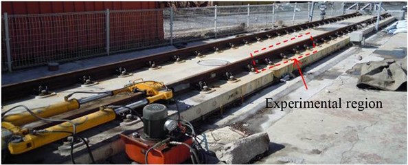
a) The test platform of ballastless track
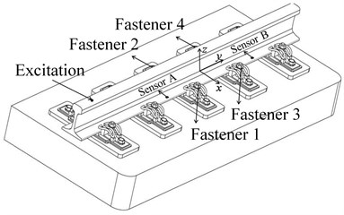
b) The schematic diagram
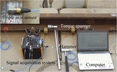
c) The experimental scene and equipments
The K-LT is an optimal orthogonal transform based on statistical feature of the object. It can eliminate the statistical correlation but retain the classified information. The state matrix is denoted by , where is the length of QTJTs, i.e., the number of valid quaternion spectra lines that participate in operation, and is the number of measured QTJTs. The covariance matrix of can be decomposed by:
where is the feature subspace spanked by the training QTJTs, and , and is the respective eigenvalue of . For each training QTJT , , it was projected to the feature subspace to get a new projection vector :
Here, projection vector was utilized as the state feature index vector. Given a pair of arbitrary testing time-domain quaternion sequences, the corresponding testing QTJT was calculated and then projected to the feature subspace to get projection vector . Thus, the testing state was just the state that contained the minimal Euclidean distance between and . The QTJTs corresponding to and are called matching QTJTs.
4. Results and discussion
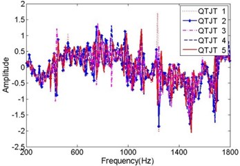
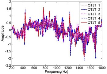
All the 20 measured QTJTs under state 1 (all fasteners tightened) were illustrated in Fig. 2, where the color code cycled every seven QTJTs and “time ” meant the -th excitation. Actually, the sampled signal usually mixed with the ambient noise and low-frequency response of the supporting structure, meanwhile, the plastic hammerhead made the power of excitation force mainly concentrate within 2 kHz. This leaded to mussy QTJTs below 0.2 kHz and beyond 1.8 kHz. Therefore, the valid frequency range was selected as 0.2 kHz-1.8 kHz in this work. The reduced QTJTs under state 1 were illustrated in Fig. 3.
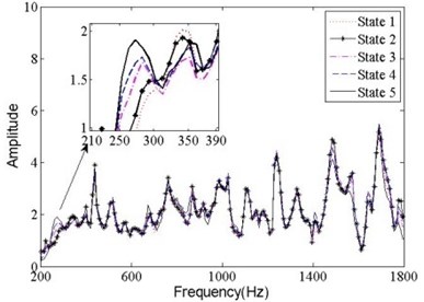
According to Eq. (3), the QTJT does not rely on the excitation force. Therefore, the QTJTs under the same state should coincide in theory. Fig. 3 indicated that all the QTJTs within valid frequency range under state 1 coincided well. If the QTJTs can be used for structural state detection, they should not only coincide under the same state but also disaccord under different states. The average QTJT under each state was calculated and illustrated in Fig. 4. Compared with Fig. 3, there were visible differences among the average QTJTs under different states. Synthesized the illustrations of Fig. 3 and Fig. 4, the QTJTs can be used for state detection really.
Fig. 2All the measured QTJTs under state 1
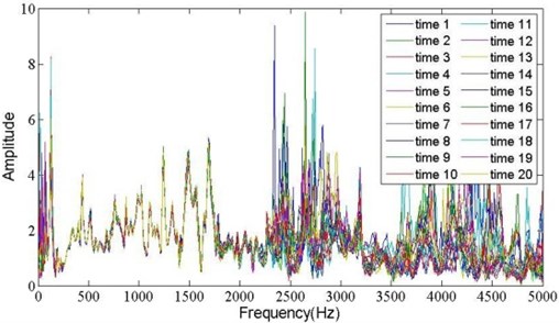
Fig. 3The reduced QTJTs under state 1
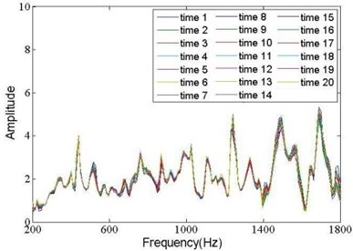
Fig. 4The average of QTJTs under different states
Furthermore, the real and imaginary components of the former five training training QTJTs under state 1 were illustrated in Fig. 5, respectively. The imaginary components of the QTJTs presented obvious distinction. But anyway, the modular vectors of the QTJTs were consistent, which was verified by Fig. 3. That was the reason why the state matrix was constructed by the modular vectors of the QTJTs rather than the QTJTs themselves.
Fig. 5The components of QTJTs in state 1
a) The real components
b) The imaginary components
c) The imaginary components
d) The imaginary components
If the vibration direction deviates the sensitive direction of the sensor, when single axis sensor is used, the vibration amplitude will decrease but the frequencies remain the same. The measured transmissibility based on scalar signals will deviate from its theoretical value unless the installation orientations of the sensors are in strict accordance with each other. However, it is difficult to strictly ensure this condition in practical applications. What is more, the vibration is usually composed from multiple dimensional synchronous vibrations whose direction may be possibly time-varying, which will result in the transmissibility varying more than simple scaling changes. At this point, state detection based on transmissibility may fall in trouble.
Fig. 6The rotation performance: a) rotation of a 3D vector v about unit vector u by an angle 2θ and b) orientation of the sensor coordinate system changed in a virtual way
a)
b)
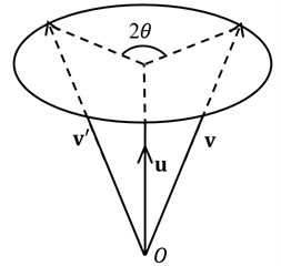
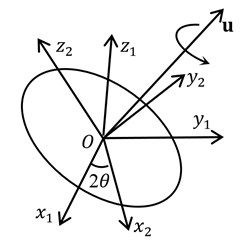
In order to verify this idea, the former five training -transmissibilities (transmissibilities based on signals from chanel) under state 1 were calculated. Subsequently, the original time-domain sequences were rotated about a 3D unit vector by employing the rotation property of quaternions. Fig. 6(a) illustrates the rotation of an arbitrary vector by an angle 2 about 3D unit vector . To extend the vector and as pure quternions by the defination mentioned in section 2. Then the rotation can be calculated by Eq. (9), where is the exponential form of a unit quaternion. It was equivalent to just rotate the sensor coordinate system about by an angle 2. In other words, the origin of the sensor coordinate system remained the same, but the orientation of the sensor coordinate system changed in a virtual way, as shown in Fig. 6(b). Without loss of generality, a rotation about vector with angle of 6 was performed for quaternion sequences from sensor . Then -tansmissibilities before and after rotation were illustrated in Fig. 7. The Fig. 7 indicated that the -transmissibilities presented distinguishing forms which were more than simple scaling changes. Furthermore, the consistency of the -transmissibilities also changed, which could be seen from the amplified subgraphs in Fig. 7. These changes also occured in -transmissibilities and -transmissibilities, which were skipped here. There was no doubt that these changes might lead to different results of state detection.
Fig. 7The former five z-transmissibility in state 1
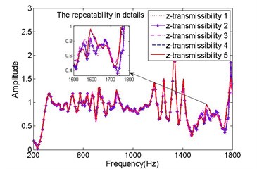
a) Before rotation
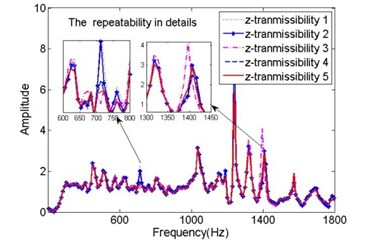
b) After rotation
When tripe axis sensor is used and its installation location is fixed, the real spatial vibration will be acquired faithfully. Obviously, the amplitude of spatial vibration at the testing point will not change with the changes of observation coordinate system. No matter how the installation orientation of the sensor changes, the variation trend of the vibration amplitude during sampling time remain the same, which can be verified by Eq. (10). As a corollary, the amplitude-frequency characteristics of the spatial vibration at testing point B remain the same, and so dose at testing point , i.e., and .
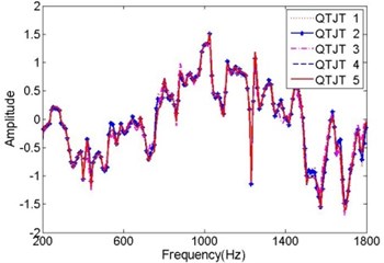
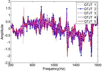
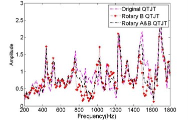
As mentioned above, only the amplitude-frequency characteristics of QTJTs were utilized in this work. According to Eq. (11), the measured QTJT (no noise is taken into consideration) should be consistent with its theoretical value in spite of the installation orientation of the sensors. Besides the rotation operation for sensor , the original time-domain quaternion sequences from sensor A were also rotated about vector with angle of 3. Thus, three QTJTs were obtained, the original QTJT, rotary QTJT and rotary A&B QTJT. It was encouraging that the QTJTs before and after rotation coincided exactly indeed, as shown in Fig. 8(a). Note that the real components and the imaginary components did not coincide before and after rotation, as shown in Fig. 8(b) and Fig. 8(c). It meant the phase-frequency characteristics of the spatial vibration changed when the sensor coordinate system changed:
Fig. 8QTJTs based on signals before and after rotation
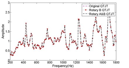
a) The integrated QTJTs
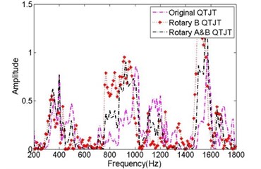
b) The real components
c) The imaginary components
According to the method mentioned in section 3, state detection was performed. As an example, the results of the first testing data from state 1 to 4 were summarized in Fig. 9. As mentioned above, the former 15 training QTJTs under each state were used as column entries to form the state matrix. That is the QTJTs of column 1 to column 15 belongs to state 1, the QTJTs of column 16 to column 30 belongs to state 2, and so on. Therefore, given a testing QTJT under state , its matching QTJT must be one of the QTJTs corresponding to column entries from to . As shown in Fig. 9, the matching QTJT of the first testing QTJT under state 1, 2, 3 and 4 is the QTJT of column 14, 28, 45, and 53, respectively. The correct detection result was obtained. The results for all the testing QTJTs were summarized in Table 1. For each testing QTJT under any state, the first column recorded the column number of its matching QTJT, and the second column recorded the result of state identification. The symbol ‘√’ meant correct identification and symbol ‘×’ meant misidentification. In this work, the suggested method resulted in a correct identification rate of 100 %.
Table 1Results of state identification for all the testing data
State No. | The serial number of matching training QTJT and identification results | |||||||||
Testing QTJT 1 | Testing QTJT 2 | Testing QTJT 3 | Testing QTJT 4 | Testing QTJT 5 | ||||||
1 | 14 | √ | 15 | √ | 14 | √ | 15 | √ | 15 | √ |
2 | 28 | √ | 27 | √ | 27 | √ | 28 | √ | 27 | √ |
3 | 45 | √ | 40 | √ | 44 | √ | 43 | √ | 45 | √ |
4 | 53 | √ | 53 | √ | 53 | √ | 53 | √ | 52 | √ |
5 | 75 | √ | 75 | √ | 71 | √ | 74 | √ | 74 | √ |
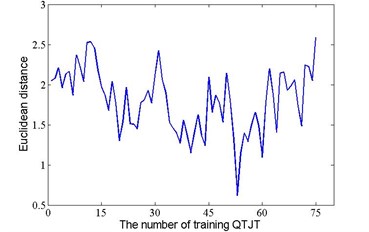
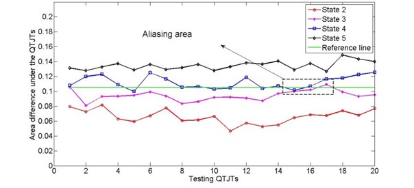
In theory, the former 15 Euclidean distances should be smaller than other ones if the testing state is state 1, Euclidean distances of 16 to 20 should be smaller than other ones if the testing state is state 2, and so on. However, the computed Euclidean distance results will generate aliasing inevitably because of multiple factors such as computing errors, tiny changes of load location and test-related uncertainty. Actually, the aliasing can be obviously seen in Fig. 8, especially between state 3 and 4. Here, magnitude state indicators proposed in Ref. [8] was also imitated by comparing the area under QTJT curves, as shown in Fig. 10. State 1 was considered as the healthy state and the green straight line was reference line, which was a free custom straight line that facilitated ordinate observation. It also presented obvious aliasing between state 3 and state 4 marked by the dashed rectangle. That was just the reason why multiple data under one state were processed and the final decision was based on the minimal Euclidean distance result.
Fig. 9The Euclidean distance between the first testing QTJT and the training QTJT
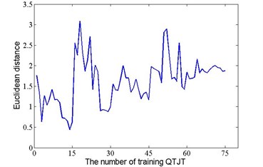
a) State 1
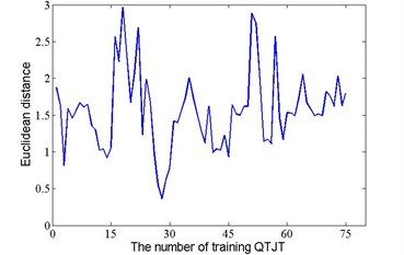
b) State 2
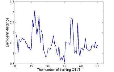
c) State 3
d) State 4
Fig. 10State indicators by comparing the area under QTJT curves
5. Conclusions
In this paper, the conventional transmissibility was promoted to quaternion field. Combined with technique of K-LT, a structural state detection method based on the QTJT was described. This method can be applied for state detection when the sampled vibration signals are composed from multiple directional vibrations and the excitation force is unavailable or inaccessible. The availability of the suggested method was demonstrated by an actual experiment on the test platform of ballastless track with single external excitation and two testing points. The result with 100 percent correct state identification was achieved. This method provides a solution to identify the presence of the state changes, but it can be further developed to identify both the presence and location of state changes by increasing the testing points and identifying the adjacent QTJTs successively. Even more important, this method preserves the theoretical value of the QTJT without specific and strict requirement for installation orientation of the sensors, which is advantageous in practical applications.
References
-
Doebling Scott W., Farrar Chareles R., Prime Michael B. A summary review of vibration-based damage identification methods. The Shock and Vibration Digest, Vol. 30, Issue 2, 1998, p. 91-105.
-
Yan Y. J., Cheng L., Wu Z. Y., Yam L. H. Development in vibration-based structural damage detection technique. Mechanical Systems and Signal Processing, Vol. 21, Issue 5, 2007, p. 2198-2211.
-
Fan W., Qiao P. Z. Vibration-based damage identification methods: a review and comparative study. Structural Health Monitoring, Vol. 10, Issue 1, 2011, p. 83-111.
-
Duan Z. D., Yan G. R., Ou J. P., Spencer B. F. Damage localization in ambient vibration by constructing proportional flexibility matrix. Journal of Sound and Vibration, Vol. 284, 2005, p. 455-466.
-
Parloo E., Verboven P., Guillaume P., van Overmeire M. Autonomous structural health monitoring – part II: vibration-based in-operation damage assessment. Mechanical Systems and Signal Processing, Vol. 16, Issue 4, 2002, p. 659-675.
-
Lu Y., Gao F. A novel time-domain auto-regressive model for structural damage diagnosis. Journal of Sound and Vibration, Vol. 283, 2005, p. 1031-1049.
-
Zhong S. C., Oyadiji S. O., Ding K. Response-only method for damage detection of beam-like structures using high accuracy frequencies with auxiliary mass spatial probing. Journal of Sound and Vibration, Vol. 311, 2008, p. 1075-1099.
-
Zhang H., Schulz M. J., Ferguson F. Structure health monitoring using transmittance functions. Mechanical Systems and Signal Processing, Vol. 13, Issue 5, 1999, p. 765-787.
-
Chen Q., Chan Y. W., Worden K. Structural fault diagnosis and isolation using neural networks based on response-only data. Computers and Structures, Vol. 81, 2003, p. 2165-2172.
-
Mao Z., Todd M. A structural transmissibility measurements-based approach for system damage detection. Proceedings of SPIE – The International Society for Optical Engineering, Vol. 7650, 2010, p. 76500G.
-
Lang Z. Q., Park G., Farrar C. R., Todd M. D., Mao Z., Zhao L., Worden K. Transmissibility of non-linear output frequency response functions with application in detection and location of damage in MDOF structural systems. International Journal of Non-Linear Mechanics, Vol. 46, 2011, p. 841-853.
-
Rehman N., Mandic D. P. Empirical mode decomposition for trivariate signals. IEEE Transactions on Signal Processing, Vol. 58, Issue 3, 2010, p. 1059-1068.
-
Yamamoto H., Aoshima N. 3D vibration-scope with quaternion processing. SICE Annual Conference in Fukui, 2003, p. 2373-2376.
-
Tong J. Feature extraction for vibration signal of asynchronous motor based on quaternion K-L transform. International Conference on Electrical and Control Engineering, 2010, p. 1006-1009.
-
Ell T. A. Hypercomplex Spectral Transforms. Ph.D. dissertation, University of Minnesota, Minneapolis, 1992.
-
Ell T. A. Quaternion-Fourier transforms for analysis of two-dimensional linear time-invariant partial-differential systems. Proceedings of 32nd IEEE Conference on Decision and Control, San Antonio, TX, Vols. 1-4, 1993, p. 1830-1841.
-
Ell T. A., Sangwine S. J. Hypercomplex fourier transforms of color images. IEEE Transactions on Image Processing, Vol. 16, Issue l, 2007, p. 22-35.
-
Moxey C. E., Sangwine S. J., Ell T. A. Hypercomplex correlation techniques for vector images. IEEE Transactions on Signal Processing, Vol. 51, Issue 7, 2003, p. 1941-1953.
About this article
This work was supported by the National Natural Science Foundation of China (No. 51305064), the Scientific Research Project of Education Department of Liaoning Province Key Laboratory, China (No. L2012014), the Fundamental Research Funds for the Central Universities, China (No. DUT13LAB14), and Open Funds of Traction Power State Key Laboratory, Southwest Jiaotong University, China (No. TPL1309).
