Theoretical study on the nonlinear behavior of a fluid micro-vibration isolator

Wang, Jie; Zhao, Shougen; Wu, Dafang

Journal of Vibroengineering

Browse Journal

Submit article

Published: 15 May 2015

Check for updates

Theoretical study on the nonlinear behavior of a fluid micro-vibration isolator

Jie Wang¹

Shougen Zhao²

Dafang Wu³

^{1, 2, 3}School of Aeronautic Science and Engineering, Beijing University of Aeronautics and Astronautics, Beijing 100191, China

Corresponding Author:

Jie Wang

Cite the article Download PDF

Downloads 1209

Abstract

Vibration isolation is an important method of spacecraft vibration control, and the study of vibration isolation performance (VIP) is the theoretical basis to design the interior structure of isolator and analyze its transmissibility characteristics. In the present study, a new type of fluid micro-vibration isolator used for space engineering is investigated, thus its nonlinear multi-parameter model whose $p$ th power damping and $q$ th power stiffness are placed in series is firstly constructed. After the application of harmonic balance method (HBM), the force and absolute displacement transmissibility curves under different parameters are obtained, and the corresponding transmissibility characteristics are estimated based on self-defined evaluation indices of VIP. Besides, the effects of some key factors, e.g., excitation amplitude and stiffness ratio, on the VIP are also analyzed. The results show that if the isolator is excited by external force in orbit, the linear model can be approximately used to analyze the VIP. However, if the isolator is excited by foundation displacement during the launch stage, only the nonlinear model can accurately describe its vibration behavior. Moreover, the numerical algorithm Runge-Kutta method is adopted to validate the above results, and a stability analysis is also carried out to show their practicability. Finally, an actual application of the nonlinear model is accomplished with the use of an optimization method called generalized pattern search (GPS) algorithm. The presented theory and method can also provide a reference and a theoretical basis for the design and engineering application of this type of fluid micro-vibration isolators.

1. Introduction

Nowadays, with the increased development of aerospace technology towards to high precision, high resolution and high stability, the vibration requirements of each component of spacecraft have become more and more rigorous during both the launch stage and the in-orbit working state. For example, with the purpose of improving the image quality and line-of-sight performance of optical payload, the vibration amplitudes of jitter sources such as momentum wheels or control momentum gyroscopes should be reduced to the order of micrometers or even nanometers [1, 2]. Active control is one type of method to attenuate the unwanted vibration but it is still imperfect on space technology aspect due to its disadvantages of costly expenditure, complex control law, additional equipment and low stability [3, 4]. Contrarily, passive control is widely employed in many countries because it has the advantages of high reliability, simple-realized principle and optimal structure format [5, 6]. Moreover, a commonly used passive method is that inserting fluid micro-vibration isolators between the disturbed components and spacecraft or/and between the optical payload and spacecraft, e.g., a type of micro-vibration isolator called D-strut was successfully used to improve the observational performance in Hubble telescope [7, 8]. Since most of micro-vibration isolators contain non-Newtonian fluid, so different flow states such as laminar flow or turbulent flow must exist in the interior structure, and they are closely related to the excitation frequency. Further, these isolators also need to experience two different periods, i.e., the launch stage and the in-orbit working state, during which the excitation types and amplitudes are significantly different. Thus the VIP always behaves nonlinearly under the complicated effects of interior structure, fluid property and external excitation, and only the nonlinear models can be used to accurately characterize the vibration isolation behavior.

As two dilemmas, i.e., the contradiction between high static stiffness and low natural frequency, and the objective between excellent VIP at high frequencies and low amplification factor at resonant region, always appear during the design of linear vibration isolators, thus more and more research interests have been turned to the nonlinear isolators. Ibrahim gave a good review about the passive nonlinear vibration isolation in reference [9]. Based on the principle of fluid mechanics, Popov et al. theoretically deduced a nonlinear orifice-type damping and analyzed its effects on the system vibration response [10]. With the use of Fourier expansion and HBM, Ravindra et al. investigated the performance of a single degree-of-freedom (DOF) model whose $p$ th power damping and $q$ th power stiffness are placed in parallel [11]. Peng et al. studied the influences of nonlinear cubic damping on a single DOF passive vibration isolation system via the HBM, and the corresponding force and displacement transmissibility curves were compared and evaluated [12]. However, Lang et al. proposed a new method called output frequency response function (OFRF) to investigate the same nonlinear model, and similar results were obtained and presented in the reference [13]. Further, Bin et al. analyzed a new type of nonlinear horizontal damping, and they compared its force and displacement VIP with that of cubic damping [14]. Zhen studied a nonlinear damping which is a hybrid function of velocity and displacement in the reference [15]. In the domain of shock isolation, Lu et al. proposed and validated a mathematical model which is called generalized Maxwell model (GMM) for a type of long-stroke damper in the seismic engineering [16]. The GMM mainly contains four parameters, i.e., stiffness coefficient, damping coefficient, stiffness exponent and damping exponent. As an accumulator housing is contained in the shock damper, the fluid elastic effect which is similar to that of a compressed balloon is vanished, thus the damping force is only proportional to the fractional exponent of velocity [17].

Based on the above review, though other types of nonlinear models, e.g., those built for shock isolators, were also extensively investigated, the nonlinear models whose damping coefficient and stiffness coefficient are placed in series because of the compressibility of fluid have not been theoretically analyzed, so it is necessary to give a comprehensive study on the VIP of fluid micro-vibration isolators to provide an insight and a proper basis for engineering applications. Thus a new type of nonlinear multi-parameter model whose $p$ th power damping and $q$ th power stiffness are placed in series is firstly constructed. Then the force and absolute displacement transmissibility curves under different parameters are obtained after the application of HBM, and the corresponding transmissibility characteristics are estimated based on self-defined evaluation indices. Further, the above results are numerically validated by the Runge-Kutta method, and a stability analysis is also carried out to show their practicability. Finally, an actual application of the nonlinear model is accomplished with the use of an optimization method called generalized pattern search (GPS) algorithm.

2. Construction and solution of the equation of motion

Fig. 1 shows the structural schematic of a fluid micro-vibration isolator, and its left and right connecting end faces are connected to the base and the isolated mass, respectively. The damping component is mainly made up of a fluid reservoir, a bellows and a damping orifice, and it is also filled up with non-Newtonian fluid silicone oil. The inner tube and the damping component form an internal path to transfer force, while the outer tube gives the other external path. If the micro-vibration isolator is excited by an external force or a foundation displacement, the silicone oil of the fluid reservoir and bellows is forced to flow to and fro through the damping orifice, thus the nonlinear damping force and nonlinear stiffness force are generated, and they mainly come from the shearing effect of the fluid in the damping orifice and the elastic deformation of the damping component. Moreover, as the analytical results shown in previous paper indicates, only the generalized nonlinear model and the complicated model can consider the effects of nonlinear damping and nonlinear stiffness, properly characterize the physical vibration and show excellent performance, but the complicated model is not convenient to use in practice [18]. As Fig. 2 shows, the nonlinear multi-parameter model of the fluid micro-vibration isolator contains stiffness coefficients $k_{1}$ , $k_{2}$ , $k_{3}$ , $k_{4}$ and a damping coefficient $c$ , the stiffness coefficient $k_{4}$ and the damping coefficient $c$ are placed in series, and then they are placed in parallel with the stiffness coefficient $k_{3}$ to form a three-parameter model which represents the damping component. Further, the stiffness coefficient $k_{2}$ of the inner tube is placed in series with the three-parameter model, and the stiffness coefficient $k_{1}$ of the outer tube is placed in parallel as the other force transferring route. Moreover, the damping exponent of $c$ and the stiffness exponent of $k_{4}$ are $p$ and $q$ , respectively. If $p = q = 1$ , this model is a linear one, but if $p > 0$ , $q > 0$ and $p \neq 1$ , $q \neq 1$ , this model is the nonlinear multi-parameter one.

Fig. 1Structural schematic of a fluid micro-vibration isolator

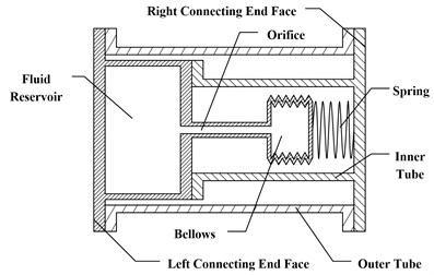
Fig. 2Nonlinear multi-parameter model of the fluid micro-vibration isolator

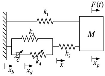
As illustrated in Fig. 2, the equation of motion of the system is:

1

\{\begin{array}{l} M {\ddot{x}}_{p} + k_{1} (x_{p} - x_{b}) + k_{2} (x_{p} - x) = F (t), \\ k_{2} (x_{p} - x) = k_{3} (x - x_{b}) + k_{4} (x - x_{d}) {|x - x_{d}|}^{q - 1}, \\ k_{4} (x - x_{d}) {|x - x_{d}|}^{q - 1} = c ({\dot{x}}_{d} - {\dot{x}}_{b}) {|{\dot{x}}_{d} - {\dot{x}}_{b}|}^{p - 1} . \end{array}

In the cases of foundation displacement excitation, $F (t) =$ 0, letting:

ω_{0} = \sqrt{k_{1} / M}, τ = ω_{0} t, x_{b} (t) = A_{1} c o s ω t,

δ_{1} (τ) = \frac{x_{p} (t) - x_{b} (t)}{A_{1}}, δ_{2} (τ) = \frac{x (t) - x_{d} (t)}{A_{1}}, δ_{3} (τ) = \frac{x (t) - x_{b} (t)}{A_{1}},

λ = \frac{ω}{ω_{0}}, N_{2} = \frac{k_{2}}{k_{1}}, N_{3} = \frac{k_{3}}{k_{1}}, N_{4} = \frac{k_{4}}{k_{1}}, ε_{1} = \frac{c A_{1}^{p - 1} ω_{0}^{p - 2}}{M},

\frac{d ()}{d t} = \frac{d ()}{d τ} \frac{d τ}{d t}, \frac{d^{2} ()}{d t^{2}} = \frac{d}{d τ} [\frac{d ()}{d τ} \frac{d τ}{d t}] \frac{d τ}{d t} .

Eq. (1) can be simplified as:

2

\{\begin{array}{l} δ_{1}^{''} (τ) + δ_{1} (τ) + N_{2} [δ_{1} (τ) - δ_{3} (τ)] = λ^{2} c o s λ τ, \\ N_{2} [δ_{1} (τ) - δ_{3} (τ)] = N_{3} δ_{3} (τ) + N_{4} A_{1}^{q - 1} δ_{2} (τ) {|δ_{2} (τ)|}^{q - 1}, \\ N_{4} A_{1}^{q - 1} δ_{2} (τ) {|δ_{2} (τ)|}^{q - 1} = ε_{1} [δ_{3}^{'} (τ) - δ_{2}^{'} (τ)] {|{δ_{3}}^{'} (τ) - δ_{2}^{'} (τ)|}^{p - 1}, \end{array}

where $A_{1}$ is the amplitude of foundation excitation, $ω$ is the excitation circular frequency and the primes denote the differentiation with respect to the non-dimensional time $τ .$

Similarly, in the cases of force excitation, $x_{b} (t) = 0,$ letting:

F (t) = F_{0} c o s ω t, ω_{0} = \sqrt{k_{1} / M}, τ = ω_{0} t, A_{2} = \frac{F_{0}}{k_{1}},

y_{1} (τ) = \frac{x_{p} (t)}{A_{2}}, y_{2} (τ) = \frac{x (t) - x_{d} (t)}{A_{2}}, y_{3} (τ) = \frac{x (t)}{A_{2}},

λ = \frac{ω}{ω_{0}}, N_{2} = \frac{k_{2}}{k_{1}}, N_{3} = \frac{k_{3}}{k_{1}}, N_{4} = \frac{k_{4}}{k_{1}}, ε_{2} = \frac{c A_{2}^{p - 1} ω_{0}^{p - 2}}{M},

the non-dimensional form of Eq. (1) is given by:

3

\{\begin{array}{l} y_{1}^{''} (τ) + y_{1} (τ) + N_{2} [y_{1} (τ) - y_{3} (τ)] = c o s λ τ, \\ N_{2} [y_{1} (τ) - y_{3} (τ)] = N_{3} y_{3} (τ) + N_{4} A_{2}^{q - 1} y_{2} (τ) {|y_{2} (τ)|}^{q - 1}, \\ N_{4} A_{2}^{q - 1} y_{2} (τ) {|y_{2} (τ)|}^{q - 1} = ε_{2} [y_{3}^{'} (τ) - y_{2}^{'} (τ)] {|y_{3}^{'} (τ) - y_{2}^{'} (τ)|}^{p - 1}, \end{array}

where $F_{0}$ is the amplitude of force excitation.

Thus Eq. (2) and Eq. (3) can be uniformly written as:

4

\{\begin{array}{l} Δ_{1}^{''} (τ) + Δ_{1} (τ) + N_{2} [Δ_{1} (τ) - Δ_{3} (τ)] = ϕ c o s λ τ, \\ N_{2} [Δ_{1} (τ) - Δ_{3} (τ)] = N_{3} Δ_{3} (τ) + N_{4} A^{q - 1} Δ_{2} (τ) {|Δ_{2} (τ)|}^{q - 1}, \\ N_{4} A^{q - 1} Δ_{2} (τ) {|Δ_{2} (τ)|}^{q - 1} = ε [Δ_{3}^{'} (τ) - Δ_{2}^{'} (τ)] {|Δ_{3}^{'} (τ) - Δ_{2}^{'} (τ)|}^{p - 1}, \end{array}

where $ϕ = λ^{2}$ and $ϕ = 1$ are for the foundation displacement excitation cases and the force excitation cases, respectively.

In order to solve the Eq. (4) analytically, the harmonic balance method (HBM) is applied without considering the sub- and super-harmonics, so the first order approximation is assumed as follows:

5

\begin{matrix} Δ_{i} (τ) = B_{i 0} + B_{i 1} c o s λ τ + B_{i 2} s i n λ τ = Z_{i 0} + Z_{i 1} c o s (λ τ + φ_{i}), \end{matrix}

where:

\{\begin{array}{l} Z_{i 0} = B_{i 0}, \\ Z_{i 1} = \sqrt{B_{i 1}^{2} + B_{i 2}^{2}}, \\ c o s φ_{i} = \frac{B_{i 1}}{\sqrt{B_{i 1}^{2} + B_{i 2}^{2}}}, \\ s i n φ_{i} = - \frac{B_{i 2}}{\sqrt{B_{i 1}^{2} + B_{i 2}^{2}}}, i = (1, 2, 3) . \end{array}

Thus $Δ_{3}^{'} (τ) - Δ_{2}^{'} (τ)$ can be expressed as:

6

\begin{matrix} Δ_{3}^{'} (τ) - Δ_{2}^{'} (τ) = (B_{21} λ - B_{31} λ) s i n λ τ + (B_{32} λ - B_{22} λ) c o s λ τ = Z_{40} + Z_{41} s i n (λ τ + φ_{4}), \end{matrix}

where:

\{\begin{array}{l} Z_{40} = 0, \\ Z_{41} = λ \sqrt{{(B_{21} - B_{31})}^{2} + {(B_{32} - B_{22})}^{2}}, \\ c o s φ_{4} = \frac{B_{21} - B_{31}}{\sqrt{{(B_{21} - B_{31})}^{2} + {(B_{32} - B_{22})}^{2}}} \\ s i n φ_{4} = \frac{B_{32} - B_{22}}{\sqrt{{(B_{21} - B_{31})}^{2} + {(B_{32} - B_{22})}^{2}}} . \end{array},

Letting $θ_{2} = λ τ + φ_{2},$ the periodic function $h (θ_{2}) = Δ_{2} (τ) {|Δ_{2} (τ)|}^{q - 1}$ can be approximated by the first order Fourier expansion as:

7

h (θ_{2}) \approx \frac{R_{20}}{2} + R_{21} c o s θ_{2} + R_{22} s i n θ_{2},

where:

R_{20} = \frac{1}{π} \int_{- π}^{+ π} h (θ_{2}) d θ_{2}, R_{21} = \frac{1}{π} \int_{- π}^{+ π} h (θ_{2}) c o s θ_{2} d θ_{2}, R_{22} = \frac{1}{π} \int_{- π}^{+ π} h (θ_{2}) s i n θ_{2} d θ_{2} .

Similarly, letting $θ_{4} = λ τ + φ_{4},$ the periodic function $h (θ_{4}) = [Δ_{3}^{'} (τ) - Δ_{2}^{'} (τ)] {|Δ_{3}^{'} (τ) - Δ_{2}^{'} (τ)|}^{p - 1}$ can also be approximately expressed as:

8

h (θ_{4}) \approx \frac{R_{40}}{2} + R_{41} c o s θ_{4} + R_{42} s i n θ_{4},

where:

R_{40} = \frac{1}{π} \int_{- π}^{+ π} h (θ_{4}) d θ_{4}, R_{41} = \frac{1}{π} \int_{- π}^{+ π} h (θ_{4}) c o s θ_{4} d θ_{4}, R_{42} = \frac{1}{π} \int_{- π}^{+ π} h (θ_{4}) s i n θ_{4} d θ_{4} .

After the mathematical integration, the values of $R_{i j}$ ( $i =$ 2, 4, $j =$ 0, 1, 2) are listed in Table 1.

Table 1The values of Rij (i= 2, 4, j= 0, 1, 2)

$R_{i j}$	$j = 0$	$j = 1$	$j = 2$
$i = 2$	0	$\frac{2}{\sqrt{π}} Z_{21}^{q} \frac{Γ ((q + 2) / 2)}{Γ ((q + 3) / 2)}$	0
$i = 4$	0	0	$\frac{2}{\sqrt{π}} Z_{41}^{p} \frac{Γ ((p + 2) / 2)}{Γ ((p + 3) / 2)}$
$Γ (\cdot)$ is the standard Gamma function.

Moreover, by setting:

ψ_{2} = \frac{2}{\sqrt{π}} \frac{Γ ((q + 2) / 2)}{Γ ((q + 3) / 2)}, ψ_{4} = \frac{2}{\sqrt{π}} \frac{Γ ((p + 2) / 2)}{Γ ((p + 3) / 2)},

the periodic functions $h (θ_{2})$ and $h (θ_{4})$ are given by:

9a

\begin{matrix} h (θ_{2}) = Z_{21}^{q} ψ_{2} c o s θ_{2} = Z_{21}^{q} ψ_{2} c o s (λ τ + φ_{2}) = Z_{21}^{q} ψ_{2} (c o s λ τ c o s φ_{2} - s i n λ τ s i n φ_{2}), \end{matrix}

9b

h (θ_{4}) = Z_{41}^{p} ψ_{4} s i n θ_{4} = Z_{41}^{p} ψ_{4} s i n (λ τ + φ_{4}) = Z_{41}^{p} ψ_{4} (s i n λ τ c o s φ_{4} + c o s λ τ s i n φ_{4}) .

Substituting the Eq. (5), Eq. (6) and Eq. (9) into Eq. (4), and equating the constant terms and the coefficients of the same harmonics on both sides of Eq. (4), then the following nonlinear equation is obtained:

10

f (B) = 0,

where:

B_{i 0} = 0, (i = 1, 2, 3), B = (\begin{array}{l} B_{11} \\ B_{12} \\ B_{21} \\ B_{22} \\ B_{31} \\ B_{32} \end{array}), f (B) = (\begin{array}{l} f_{1} (B) \\ f_{2} (B) \\ f_{3} (B) \\ f_{4} (B) \\ f_{5} (B) \\ f_{6} (B) \end{array}) .

By setting:

D_{1} = {(B_{21}^{2} + B_{22}^{2})}^{\frac{q - 1}{2}}, D_{3} = {[{(B_{21} - B_{31})}^{2} + {(B_{32} - B_{22})}^{2}]}^{\frac{p - 1}{2}},

$f (B)$ can be rewritten as:

11

f (B) = (\begin{matrix} (1 - λ^{2} + N_{2}) B_{11} - N_{2} B_{31} - ϕ \\ (1 - λ^{2} + N_{2}) B_{12} - N_{2} B_{32} \\ N_{2} B_{11} - (N_{2} + N_{3}) B_{31} - N_{4} A^{q - 1} ψ_{2} B_{21} D_{1} \\ N_{2} B_{12} - (N_{2} + N_{3}) B_{32} - N_{4} A^{q - 1} ψ_{2} B_{22} D_{1} \\ N_{4} A^{q - 1} ψ_{2} B_{21} D_{1} - ε λ^{p} ψ_{4} (B_{32} - B_{22}) D_{3} \\ N_{4} A^{q - 1} ψ_{2} B_{22} D_{1} - ε λ^{p} ψ_{4} (B_{21} - B_{31}) D_{3} \end{matrix}) .

Further, the Newton-Raphson method is used to solve the Eq. (10), thus the amplitude vector $B$ and the corresponding non-dimensional variables $Δ_{i} (τ)$ ,i= (1, 2, 3) can be easily obtained.

3. Evaluation indices of VIP

In the cases of foundation displacement excitation, the absolute displacement transmissibility is defined as the ratio of the amplitude of absolute displacement to that of foundation displacement. As can be seen from Eq. (4), the non-dimensional form of absolute displacement $δ_{p a} (τ)$ is given by:

12

δ_{p a} (τ) = Δ_{1} (τ) + c o s λ τ,

thus the absolute displacement transmissibility $T_{d}$ can be written as:

13

T_{d} = \sqrt{{(B_{11} + 1)}^{2} + B_{12}^{2}} .

In the cases of force excitation, the force transmissibility is defined as the ratio of the amplitude of the force transmitted into the foundation to that of excitation force. Similarly, the non-dimensional form of the force transmitted into the foundation $F_{t}$ can be expressed as:

14

F_{t} = Δ_{1} (τ) + N_{2} [Δ_{1} (τ) - Δ_{3} (τ)] = Δ_{1} (τ) + N_{3} Δ_{3} (τ) + N_{4} A^{q - 1} Δ_{2} (τ) {|Δ_{2} (τ)|}^{q - 1}

= Δ_{1} (τ) + N_{3} Δ_{3} (τ) + ε [Δ_{3}^{'} (τ) - Δ_{2}^{'} (τ)] {|Δ_{3}^{'} (τ) - Δ_{2}^{'} (τ)|}^{p - 1},

thus the force transmissibility $T_{f}$ is given by:

15

T_{f} = \sqrt{B_{11}^{2} + B_{12}^{2}} + N_{3} \sqrt{B_{31}^{2} + B_{32}^{2}} + N_{4} A^{q - 1} {[B_{21}^{2} + B_{22}^{2}]}^{\frac{q}{2}} .

In general, the following indices are considered in this paper to evaluate the VIP, namely, (1) the peak value of transmissibility, i.e., the maximum value of force transmissibility $T_{f r}$ and the maximum value of absolute displacement transmissibility $T_{d r};$ (2) the non-dimensional resonant frequency $λ_{r}$ , at which the peak value of transmissibility appears; (3) the absolute value of the slope of transmissibility curve at high frequencies which are above the resonant frequency $λ_{r}$ , i.e. the high frequency roll-off rate HFRR. Further, another index called non-dimensional frequency shift rate $λ_{ν}$ is defined as follows:

16

λ_{ν} = \frac{λ_{r} - λ_{0}}{λ_{0}} \times 100 %,

where $λ_{0}$ is the non-dimensional frequency which corresponds to the circular frequency $ω_{0}$ and its value is $λ_{0} = 1.$

4. Stability analysis

As the nonlinear damping force and nonlinear restoring force have no continuous derivatives with respect to $B_{i j}$ ( $i =$ 2, 3, $j =$ 0, 1, 2), thus a stability analysis procedure stated in reference [11] is adopted in this paper. First, we assume that the vibration amplitude vector $B$ varies with the non-dimensional time $τ$ slowly, thus the corresponding second order derivatives can be neglected. After substituting the Eq. (5), Eq. (6) and Eq. (9) into Eq. (4), taking a differentiation with respect to $τ$ in the second and third formulas, and equating the coefficients of the same harmonics on both sides of Eq. (4), then the following autonomous equation can be obtained:

17a

\{\begin{array}{l} B_{11}^{'} = \frac{1}{(2 λ)} [(1 + N_{2} - λ^{2}) B_{12} - N_{2} B_{32}], \\ B_{12}^{'} = \frac{1}{(2 λ)} [ϕ + (λ^{2} - 1 - N_{2}) B_{11} + N_{2} B_{31}], \end{array}

17b

[\begin{array}{l} H_{11} & H_{12} & H_{13} & H_{14} \\ H_{21} & H_{22} & H_{23} & H_{24} \\ H_{31} & H_{32} & H_{33} & H_{34} \\ H_{41} & H_{42} & H_{43} & H_{44} \end{array}] [\begin{array}{l} B_{21}^{'} \\ B_{22}^{'} \\ B_{31}^{'} \\ B_{32}^{'} \end{array}] = [\begin{array}{l} g_{1} \\ g_{2} \\ g_{3} \\ g_{4} \end{array}],

where $H_{i j}$ ( $i =$ 1, 2, 3, 4, $j =$ 1, 2, 3, 4), $g_{i}$ ( $i =$ 1, 2, 3, 4) are given in the Appendix and $B_{i j}^{'}$ ( $i =$ 2, 3, $j =$ 1, 2) can be obtained by solving the linear Eq. (17b). Letting $B_{i j}^{'} = 0$ ( $i =$ 1, 2, 3, $j =$ 1, 2), each balance point $B_{i j}^{0}$ ( $i =$ 1, 2, 3, $j =$ 1, 2) at different frequencies can also be found, and the corresponding stability property is investigated by considering the following linearized equation:

18

U' = J_{U} U,

where $U = {[\begin{array}{l} \begin{array}{l} \begin{array}{l} U_{11} & U_{12} \end{array} & U_{21} \end{array} & U_{22} & U_{31} & U_{32} \end{array}]}^{T},$ $B_{i j} = B_{i j}^{0} + U_{i j}$ ( $i =$ 1, 2, 3, $j =$ 1, 2), $J_{U}$ is the jacobian matrix of the system under consideration. If the eigenvalues of $J_{U}$ have negative real components, the solution is always stable. But in this paper, as some eigenvalues have conjugated pure imaginaries, thus another preliminary stability analysis is carried out by integrating the above autonomous Eq. (17) with different initial conditions to obtain the phase plot.

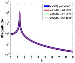
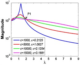
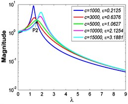
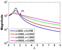
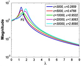
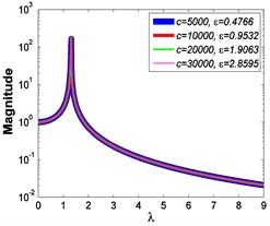
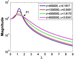
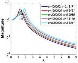
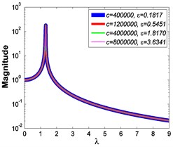
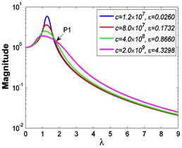
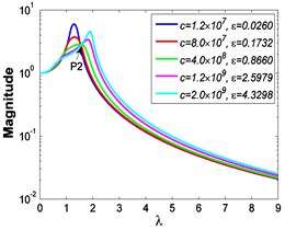
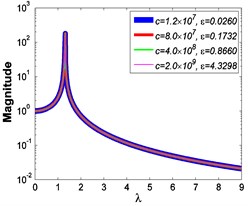
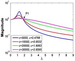
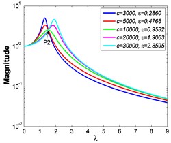
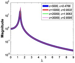
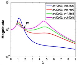
Fig. 3Force transmissibility curves under F0= 50 N

a1) $p = 0.6, q = 0.6$

b1) $p = 0.6, q = 1$

c1) $p = 0.6, q = 1.5$

a2) $p = 0.85, q = 0.6$

b2) $p = 0.85, q = 1$

c2) $p = 0.85, q = 1.5$

a3) $p = 1, q = 0.6$

b3) $p = 1, q = 1$

c3) $p = 1, q = 1.5$

a4) $p = 2, q = 0.6$

b4) $p = 2, q = 1$

c4) $p = 2, q = 1.5$

a5) $p = 3, q = 0.6$

b5) $p = 3, q = 1$

c5) $p = 3, q = 1.5$

5. Results and discussion

For the nonlinear model studied in this paper, the following parameter values, i.e., $M = 30 kg,$ $k_{1} =$ 3.669×10⁶ N/m, $k_{2} =$ 1.191×10⁸ N/m, $k_{3} =$ 2.482×10⁶ N/m and $k_{4} =$ 8.928×10⁶ N/m^q, are used to obtain the transmissibility curves.

5.1. Force excitation cases

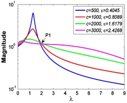
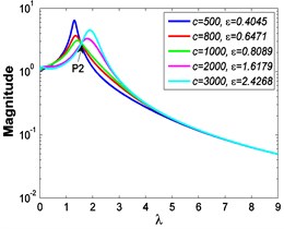
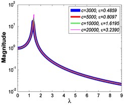
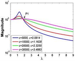
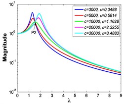
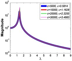
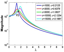
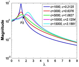
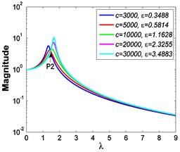
Fig. 3 shows the force transmissibility curves when $F_{0} =$ 50 N.

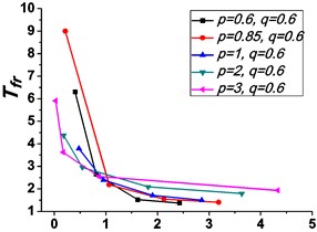
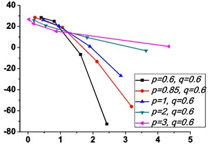
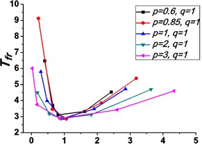
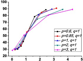
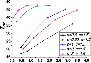
Fig. 4 shows the variations of the peak value of force transmissibility $T_{f r}$ and the non-dimensional frequency shift rate $λ_{ν}$ with damping ratio $ε$ .

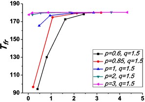
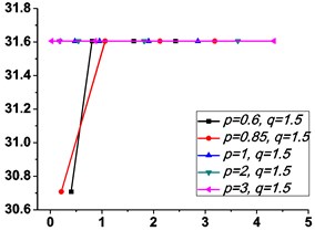
Fig. 4Variations of the peak value of force transmissibility Tfr and the non-dimensional frequency shift rate λν with damping ratio ε

a1) $q =$ 0.6

b1) $q =$ 0.6

a2) $q =$ 1

b2) $q =$ 1

a3) $q =$ 1.5

b3) $q =$ 1.5

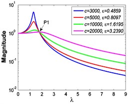
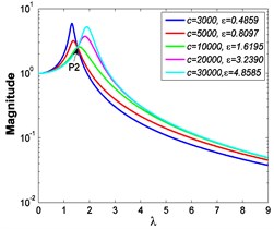
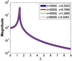
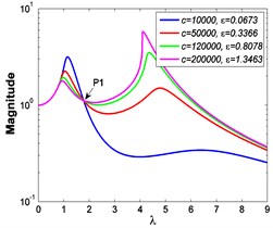
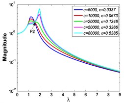
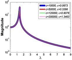
As illustrated in Fig. 3 and Fig. 4, the stiffness exponent $q$ has significant effects on the VIP in the considered scope of damping ratio $ε$ . (1) If $q =$ 0.6, as shown in Fig. 3(a1)-(a5), Fig. 4(a1) and Fig. 4(b1), only one resonant region is included and all of the transmissibility curves approximately pass through one common point $P_{1}$ . With the increase of damping ratio $ε$ , the resonant frequency $λ_{r}$ shifts towards left, the peak value of transmissibility $T_{f r}$ reduces, and the high frequency roll-off rate $H F R R$ decreases. Besides, if the damping exponent $p$ is large, e.g. $p =$ 3, the system changes more slowly with the increase of damping ratio $ε$ , and the high frequency roll-off rates $H F R R s$ under different damping ratios are much easier to become consistent with each other, thus the variation extent of force transmissibility curves drops a lot. (2) If $q =$ 1, as shown in Fig. 3(b1)-(b5), Fig. 4(a2) and Fig. 4(b2), similarly to the linear five-parameter model, two resonant regions are included and separated by one common point $P_{2}$ , which is the critical point between the first resonant region on the left hand side and the second resonant region on the right hand side. With the increase of damping ratio $ε$ , the resonant frequency $λ_{r}$ gradually shifts from the first resonant region to the second one, while the resonant peak $T_{f r}$ firstly reduces to the point $P_{2}$ and then goes up. If the resonant frequency $λ_{r}$ is at the first resonant region, the high frequency roll-off rate HFRR decreases with the rise of damping ratio $ε$ , but there is an opposite situation if the resonant frequency $λ_{r}$ is at the second resonant region. Besides, if $λ \geq$ 4, the variations of high frequency roll-off rates HFRRs tend to the same and become nearly independent on the damping ratio $ε$ . Further, the smaller the damping exponent $p$ is, the faster the variations of resonant peak $T_{f r}$ and frequency shift rate $λ_{ν}$ with damping ratio $ε$ are, thus the transmissibility curves become much easier to transfer from the first resonant region to the second one. (3) If $q =$ 1.5, as shown in Fig. 3(c1)-(c5), Fig. 4(a3) and Fig. 4(b3), only one resonant region is included. Since the severe rigid effect of the stiffness coefficient $k_{4}$ , the variation of frequency shift rate $λ_{ν}$ is small and the resonant peak $T_{f r}$ is very high. It can also be seen that the damping ratio $ε$ nearly only affects the peak value of transmissibility $T_{f r}$ , and the shape of force transmissibility curves is almost unchanged. Furthermore, the larger the damping exponent $p$ is, the larger the resonant peak $T_{f r}$ is, but the smaller the variation extent of frequency shift rate $λ_{ν}$ is.

5.2. Foundation displacement excitation cases

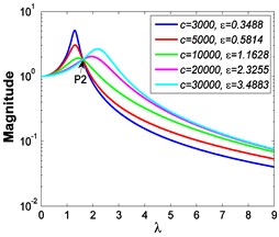
Fig. 5 shows the absolute displacement transmissibility curves when $A =$ 7.599×10^-4 m.

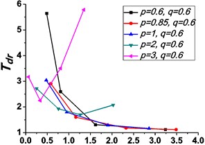
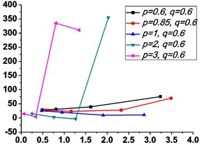
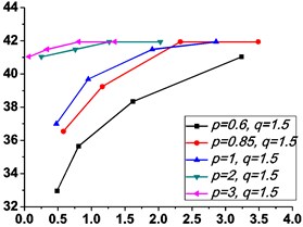
Fig. 6 illustrates the variations of the peak value of absolute displacement transmissibility $T_{d r}$ and the non-dimensional frequency shift rate $λ_{ν}$ with damping ratio $ε$ .

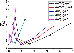
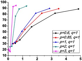
Similarly, it can be seen from Fig. 5 and Fig. 6 that the stiffness exponent $q$ has significant effects on the VIP in the considered scope of damping ratio $ε$ . (1) If $q =$ 0.6, as illustrated in Fig. 5(a1)-(a5), Fig. 6(a1) and Fig. 6(b1), all of the transmissibility curves approximately pass through one common point $P_{1}$ . If $p \leq$ 1, only one resonant region is included, but two resonant regions which are separated by the point $P_{1}$ appear in other situations. If $p = 0.6$ or 0.85, the resonant frequency $λ_{r}$ shifts towards to high frequency with the increase of damping ratio $ε$ , but an opposite situation occurs if the damping exponent $p$ is equal to one. Besides, an increased damping ratio $ε$ can lead to the resonant peak $T_{d r}$ and the high frequency roll-off rate HFRR decrease. If $p =$ 2 or 3, the resonant frequency $λ_{r}$ and the corresponding resonant peak $T_{d r}$ firstly drop down and then rise with the increase of damping ratio $ε$ , but it should be noted that the VIP becomes unacceptable due to the large second resonant frequency. Moreover, the larger the damping exponent $p$ is, the larger the variation extents of resonant peak $T_{d r}$ and frequency shift rate $λ_{ν}$ are, thus the transmissibility curves change more obviously with damping ratio $ε$ . (2) If $q = 1$ and $p =$ 2 or 3, as shown in Fig. 5(b1)-(b5) and Fig. 6(a2) and Fig. 6(b2), the resonant frequency $λ_{r}$ shifts towards left at the beginning and then transfers from the first resonant region to the second one. Besides, the resonant peak $T_{d r}$ decreases firstly and then goes up under the influences of an increased damping ratio $ε$ . The larger the damping exponent $p$ is, the smaller the resonant peak $T_{d r}$ is at the first resonant region, but this variation becomes different at the second resonant region. Further, the larger the damping exponent $p$ is, the faster the variation of frequency shift rate $λ_{ν}$ is, thus the transmissibility curves are much easier to transfer from the first resonant region to the second one. Other variations are similar to that of force excitation cases except the magnitudes are different, thus they will not be repeated again. (3) If $q =$ 1.5, as illustrated in Fig. 5(c1)-(c5), Fig. 6(a3) and Fig. 6(b3), the effects of damping ratio $ε$ and damping exponent $p$ are similar to that of force excitation cases, and the performance of isolator is mainly determined by the stiffness exponent $q$ .

Fig. 5Absolute displacement transmissibility curves under A= 7.599×10-4 m

a1) $p = 0.6, q = 0.6$

b1) $p = 0.6, q = 1$

c1) $p = 0.6, q = 1.5$

a2) $p = 0.85, q = 0.6$

b2) $p = 0.85, q = 1$

c2) $p = 0.85, q = 1.5$

a3) $p = 1, q = 0.6$

b3) $p = 1, q = 1$

c3) $p = 1, q = 1.5$

a4) $p = 2, q = 0.6$

b4) $p = 2, q = 1$

c4) $p = 2, q = 1.5$

a5) $p = 3, q = 0.6$

b5) $p = 3, q = 1$

c5) $p = 3, q = 1.5$

Fig. 6Variations of the peak value of absolute displacement transmissibility Tdr and the non-dimensional frequency shift rate λν with damping ratio ε

Variations of the peak value of absolute displacement transmissibility Tdr and the non-dimensional frequency shift rate λν with damping ratio ε

a1) $q =$ 0.6

b1) $q =$ 0.6

a2) $q =$ 1

b2) $q =$ 1

a3) $q =$ 1.5

b3) $q =$ 1.5

5.3. Effects of excitation amplitude

As shown in Eq. (4), different excitation amplitudes have distinct effects on the VIP. Since the micro-vibration isolator studied in this paper needs to survive from the launch stage and experience the in-orbit working state, thus the corresponding maximum values of foundation excitation amplitude and force excitation amplitude are set as $A =$ 5.066×10^-3 m and $F_{0} =$ 100 N, respectively. Similarly, as the nonlinear stiffness effect is weak, the damping exponent and the stiffness exponent are set as $p =$ 0.85 and $q =$ 1, respectively. Fig. 7 shows the comparative force transmissibility curves when $F_{0} =$ 50 N and $F_{0} =$ 100 N.

Fig. 7Force transmissibility curves

a) $F_{0} =$ 50 N

b) $F_{0} =$ 100 N

As illustrated in Fig. 7, if the isolator is excited by external force in orbit and keeps the same damping coefficient $c$ , a smaller excitation amplitude $F_{0}$ can cause a larger damping ratio $ε$ and a faster frequency shift rate $λ_{r}$ , thus the transmissibility curves shift more easily from the first resonant region to the second one. Further, as shown in Fig. 3 and Fig. 4, if $q =$ 1, the variations of VIP are nearly the same when $p =$ 0.85 and $p =$ 1. Besides, since the vibration amplitude of micro-vibration isolators in orbit is of the order of micrometers or even nanometers, different excitation amplitudes have small influences on the VIP, thus a linear model can be approximately used to evaluate the force transmissibility characteristics.

Fig. 8 shows the comparative absolute displacement transmissibility curves when $A =$ 7.599×10^-4 m and $A =$ 5.066×10^-3 m.

Similarly, as shown in Fig. 8, if the micro-vibration isolator is excited by foundation displacement and keeps the same damping coefficient $c$ during the launch stage, the smaller the excitation amplitude $A$ is, the larger the damping ratio $ε$ and the frequency shift rate $λ_{r}$ are, thus the transmissibility curves transfer more easily from the first resonant region to the second one. As indicated in Fig. 5 and Fig. 6, if $q =$ 1, the VIP is seriously affected by different damping exponents $p$ . Further, since the foundation excitation amplitude is relatively large during the launch stage, thus the effects of nonlinear factors should be considered carefully by using the nonlinear model.

Fig. 8Absolute displacement transmissibility curves

a) $A =$ 7.599×10^-4 m

b) $A =$ 5.066×10^-3 m

5.4. Effects of stiffness ratio $N_{4}$

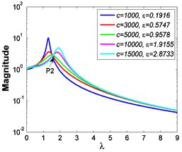
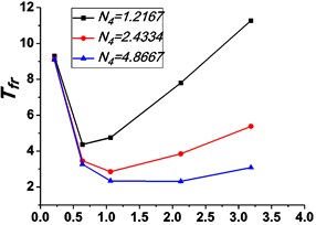
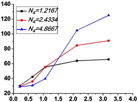
If $p =$ 0.85, $q =$ 1 and $F_{0} =$ 50 N, Fig. 9 shows the force transmissibility curves under different stiffness ratios $N_{4}$ , and Fig. 10 shows the corresponding variations of the peak value of force transmissibility $T_{f r}$ and the non-dimensional frequency shift rate $λ_{ν}$ with damping ratio $ε$ .

Fig. 9Force transmissibility curves

a) $N_{4} =$ 1.2167

b) $N_{4} =$ 2.4334

c) $N_{4} =$ 4.8667

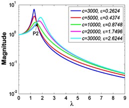
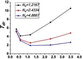
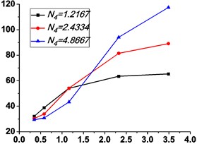
If $p =$ 0.85, $q =$ 1 and $A =$ 7.599×10^-4 m, Fig. 11 shows the absolute displacement transmissibility curves under different stiffness ratios $N_{4}$ , and Fig. 12 shows the corresponding variations of the peak value of absolute displacement transmissibility $T_{d r}$ and the non-dimensional frequency shift rate $λ_{ν}$ with damping ratio $ε$ .

As shown in Figs. 9-12, the variations of force and absolute displacement transmissibility curves with stiffness ratio $N_{4}$ are the same. With the increase of stiffness ratio $N_{4}$ , the second resonant frequency increases obviously as expected, and the variation extent of resonant peak $T_{f r}$ or $T_{d r}$ reduces, but that of frequency shift rate $λ_{ν}$ rises. Moreover, the variation extent of high frequency roll-off rate $H F R R$ also increases with an increased stiffness ratio $N_{4}$ .

Fig. 10Variations of the peak value of force transmissibility Tfr and the non-dimensional frequency shift rate λν with damping ratio ε

a)

b)

Fig. 11Absolute displacement transmissibility curves

a) $N_{4} =$ 1.2167

b) $N_{4} =$ 2.4334

c) $N_{4} =$ 4.8667

Fig. 12Variations of the peak value of absolute displacement transmissibility Tdr and the non-dimensional frequency shift rate λν with damping ratio ε

a)

b)

5.5. Numerical validation

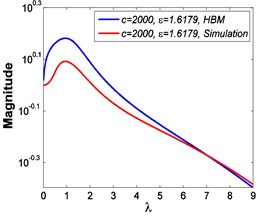
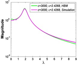
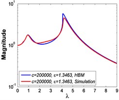
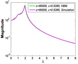
In order to validate the effectiveness of the above results, the numerical algorithm Runge-Kutta method is applied to solve the Eq. (4), some typical cases are chosen and simulated, and the corresponding force and absolute displacement transmissibility curves are shown in Fig. 13 and Fig. 14, respectively.

It can be seen from Fig. 13 and Fig. 14 that the simulated results and those obtained by HBM have small differences, and the relative errors mainly come from the numerical calculation and strong nonlinear effect. However, in the cases of weak nonlinear effect, e.g. the micro-vibration isolator studied in this paper $p =$ 0.85, $q =$ 1, they always agree with each other very well. Further, a frequency spectrum analysis is carried out for the numerical results obtained by Runge-Kutta method to illustrate the feasibility of HBM, and an evaluation index is defined as follows:

19

R e s = \frac{Q_{s}}{Q_{t}} \times 100 %,

where $Q_{s}$ is the magnitude of the sub-harmonics, the super-harmonics or the principal harmonic, and $Q_{t}$ is the total magnitude of all the harmonics. Besides, some analytical results in the force excitation cases and foundation excitation cases are shown in Table 2 and Table 3, respectively.

Table 2The results of frequency spectrum analysis in the force excitation cases

Analysis cases	Sub-harmonics	Principal harmonic at excitation frequency	Super-harmonics
$p = 0.6, q = 0.6,$ $c = 3000, ε = 2.4268$	$λ < 0.292$	$λ = 0.292$	$λ > 0.292$
	$\approx 0$ %	$\approx 100 %$	$\approx 0 %$
	$λ < 1.285$	$λ = 1.285$	$λ > 1.285$
	$\approx 0$ %	$\approx 85 %$	$\approx 15 %$
	$λ < 4$	$λ = 4$	$λ > 4$
	$\approx 0 %$	$\approx 90 %$	$\approx 10 %$
$p = 0.6, q = 1,$ $c = 3000, ε = 2.4268$	$λ < 1.303$	$λ = 1.303$	$λ > 1.303$
	$\approx 0 %$	$\approx 100 %$	$\approx 0 %$
	$λ < 1.891$	$λ = 1.891$	$λ > 1.891$
	$\approx 0 %$	$\approx 100 %$	$\approx 0 %$
	$λ < 5$	$λ = 5$	$λ > 5$
	$\approx 0 %$	$\approx 100 %$	$\approx 0 %$
$p = 0.6, q = 1.5,$ $c = 3000, ε = 2.4268$	$λ < 0.5$	$λ = 0.5$	$λ > 0.5$
	$\approx 0 %$	$\approx 50 %$	$\approx 50 %$
	$λ < 1.316$	$λ = 1.316$	$λ > 1.316$
	$\approx 0 %$	$\approx 100 %$	$\approx 0 %$
	$λ < 4$	$λ = 4$	$λ > 4$
	$\approx 50 %$	$\approx 50 %$	$\approx 0 %$

Table 3The results of frequency spectrum analysis in the foundation excitation cases

Analysis cases	Sub-harmonics	Principal harmonic at excitation frequency	Super-harmonics
$p = 3, q = 0.6,$ $c = 200000, ε = 1.3463$	$λ < 3$	$λ = 3$	$λ > 3$
	$\approx 0 %$	$\approx 100 %$	$\approx 0 %$
	$λ < 4.105$	$λ = 4.105$	$λ > 4.105$
	$\approx 0 %$	$\approx 100 %$	$\approx 0 %$
	$λ < 6$	$λ = 6$	$λ > 6$
	$\approx 0 %$	$\approx 100 %$	$\approx 0 %$
$p = 3, q = 1,$ $c = 80000, ε = 0.5385$	$λ < 1$	$λ = 1$	$λ > 1$
	$\approx 0 %$	$\approx 100 %$	$\approx 0 %$
	$λ < 1.949$	$λ = 1.949$	$λ > 1.949$
	$\approx 0 %$	$\approx 100 %$	$\approx 0 %$
	$λ < 4$	$λ = 4$	$λ > 4$
	$\approx 0 %$	$\approx 100 %$	$\approx 0 %$
$p = 3, q = 1.5,$ $c = 200000, ε = 1.3463$	$λ < 0.5$	$λ = 0.5$	$λ > 0.5$
	$\approx 0 %$	$\approx 100 %$	$\approx 0 %$
	$λ < 1.419$	$λ = 1.419$	$λ > 1.419$
	$\approx 0 %$	$\approx 100 %$	$\approx 0 %$
	$λ < 4$	$λ = 4$	$λ > 4$
	$\approx 0 %$	$\approx 100 %$	$\approx 0 %$

Fig. 13Force transmissibility curves under F0= 50 N

a) $p = 0.6, q = 0.6$

b) $p = 0.6, q = 1$

Fig. 14Absolute displacement transmissibility curves under A= 7.599×10-4 m

a) $p = 3, q = 0.6$

b) $p = 3, q = 1$

As illustrated in Table 2 and Table 3, though the magnitude of the sub-harmonics or the super-harmonics accounts for a large percent in some cases where strong nonlinear effect happens, however, only the principal harmonic appears in the most of excitation cases. Thus, these results further prove the effectiveness and feasibility of HBM to investigate the VIP of this type of nonlinear models whose nonlinear damping and nonlinear stiffness are placed in series.

5.6. Stability analysis

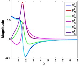
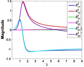
As described in Section 4, each balance point $B_{i j}^{0}$ ( $i =$ 1, 2, 3, $j =$ 1, 2) at different frequencies can be obtained by solving the equation $B_{i j}^{'} = 0$ ( $i =$ 1, 2, 3, $j =$ 1, 2). Fig. 15 shows the variations of each balance point $B_{i j}^{0}$ ( $i =$ 1, 2, 3, $j =$ 1, 2) with excitation frequency in different cases.

Fig. 15Variations of each balance point with excitation frequency: a) F0= 50 N, b) A= 7.599×10-4 m

a) $p = 0.85, q = 1, c = 5000$

b) $p = 1, q = 0.6, c = 10000$

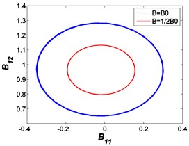
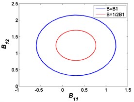
After integrating the autonomous Eq. (17) with respective initial conditions $B_{0} =$ [0 0.9 0.4 0.3 0 0.9] and $B_{1} =$ [0.3 1.3 0 0.1 0.2 1.2], the following ellipses between $B_{11}$ and $B_{12}$ can be obtained.

As illustrated in Fig. 16, it can be seen that the balance points are at the central position, thus these balance points are always stable and the corresponding solutions are effective. But if strong nonlinear effect which is caused by large damping coefficient, nonlinear exponents and large excitation amplitude appears, such as some $q =$ 1.5 and $q =$ 0.6 cases, the corresponding balance points and solutions may become unstable in these situations.

Fig. 16Ellipses between B11 and B12: a) F0= 50 N, b) A= 7.599×10-4 m

a) $λ = 1.563$

b) $λ = 1.200$

5.7. Actual application

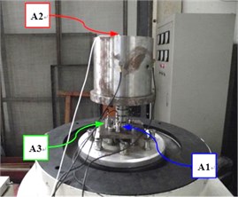
As stated in section 5.3, if the micro-vibration isolator is excited by external force in orbit, the linear model can be approximately used to analyze its VIP. However, the nonlinear model shown in Fig. 2 should be applied to consider the effects of nonlinear factors if the isolator is excited by foundation displacement during the launch stage. Further, in order to identify the nonlinear model parameters and obtain an actual application, the test set-up shown in Fig. 17 is built and used to measure the absolute displacement transmissibility curves. It is mainly made up of a shaking table, a controller, a data acquisition and analysis system, a large mass, accelerometer sensors A1, A2 and A3, etc. The accelerometer sensors A1 and A2 are used to measure the input foundation excitation and the output of the large mass, respectively. Then these two signals are sampled by the data acquisition and analysis system, and the corresponding transmissibility curves can be obtained after a data process. Moreover, the output of the shaking table is also controlled and measured by the controller and the accelerometer sensor A3, respectively. Thus a closed loop between them is formed to ensure the stability and security of excitation. Fig. 18 is a picture of the test set-up of foundation excitation.

Fig. 17The schematic diagram of the test setup of foundation excitation

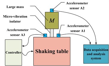
Fig. 18A picture of the test setup of foundation excitation

The GPS algorithm of Matlab optimization toolbox is adopted to identify the damping coefficient $c$ and the stiffness coefficient $k_{4}$ , and the objective function is defined as:

20

M i n i m i z e J = \sqrt{\frac{1}{P} \sum_{i = 1}^{P} (T_{d, c o m} [i] - T_{d, e x p} [i])^{2}},

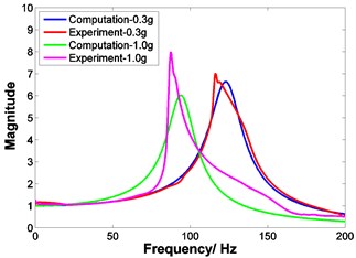
where $P$ is the number of comparative frequency points at which both the experimental absolute displacement transmissibility $T_{d, e x p} [i]$ and the corresponding computational transmissibility $T_{d, c o m} [i]$ are evaluated. Moreover, other parameters, i.e., $M =$ 30 kg, $k_{1} =$ 3.669×10⁶ N/m, $k_{2} =$ 1.191×10⁸ N/m, $k_{3} =$ 2.482×10⁶ N/m, $p =$ 0.85 and $q =$ 1, are given, and an initial parameter point of $c$ and $k_{4}$ is assumed to start the iterative identification procedure. As there is no need of derivatives or gradients, thus this algorithm is suitable for complex optimization problems which have non-differentiable or even non-continuous objective functions [16]. With the use of the identified parameters, the finally computational transmissibility is obtained and compared with that of experiment. As illustrated in Fig. 19, if the excitation amplitude is 0.3 g (1 g $=$ 10 m/s²), the computational transmissibility and the tested data are consistent with each other. However, if the excitation amplitude is 1.0 g, the differences of the magnitude of transmissibility appear slightly.

Fig. 19Absolute displacement transmissibility curves

6. Conclusions

This paper mainly studied a type of fluid micro-vibration isolator used for space engineering. As it needs to survive from the launch stage and experience the in-orbit working state, the VIP always behaves nonlinearly under the complex effects of external excitation, fluid property and interior structure. With the application of HBM, a nonlinear multi-parameter model whose $p$ th power damping and $q$ th power stiffness are placed in series is analyzed, and the corresponding force and absolute displacement transmissibility curves under different parameters are obtained. Then the related transmissibility characteristics are estimated based on self-defined evaluation indices, and the effects of key factors, e.g. excitation amplitude and stiffness ratio, are also analyzed. If the isolator is excited by external force in orbit, the linear model can be approximately used to obtain the VIP. However, if the isolator is excited by foundation displacement during the launch stage, the nonlinear effects can only be considered by using the nonlinear model. Moreover, the numerical algorithm Runge-Kutta method is adopted to validate the above results, and a stability analysis is also carried out to show their practicability. Finally, an actual application of the nonlinear model is accomplished with the use of an optimization method called generalized pattern search (GPS) algorithm. The presented theory and method can also provide a reference and a theoretical basis for the design and engineering application of this type of fluid micro-vibration isolators.

References

Cobb R. G., Sullivan J. M., Das A., et al. Vibration isolation and suppression system for precision payloads in space. Smart Materials and Structures, Vol. 8, Issue 6, 1999, p. 798-812.

Search CrossRef
Inamori T., Wang J., Saisutjarit P., et al. Jitter reduction of a reaction wheel by management of angular momentum using magnetic torquers in nano-and micro-satellites. Advances in Space Research, 2013, p. 222-231.

Search CrossRef
Foshage G. K., Davis T., Sullivan J. M., et al. Hybrid active/passive actuator for spacecraft vibration isolation and suppression. SPIE’s International Symposium on Optical Science, Engineering, and Instrumentation. International Society for Optics and Photonics, 1996.

Search CrossRef
Vaillon L., Petitjean B., Frapard B., et al. Active isolation in space truss structures: from concept to implementation. Smart Materials and Structures, Vol. 8, Issue 6, 1999, p. 781-790.

Search CrossRef
Rittweger A., Albus J., Hornung E., et al. Passive damping devices for aerospace structures. Acta Astronautica, Vol. 50, Issue 10, 2002, p. 597-608.

Search CrossRef
Liu Tian-xiong, Lin Yi-ming, Wang Ming-yu, et al. Review of the spacecraft vibration control technology. Journal of Astronautics, Vol. 29, Issue 1, 2008, p. 1-12, (in Chinese).

Search CrossRef
Davis L. P., Carter D. R., Hyde T. T. Second-generation hybrid D-strut. Smart Structures and Materials’. International Society for Optics and Photonics, 1995.

Search CrossRef
Davis P., Cunningham D., Harrell J. Advanced 1.5 Hz passive viscous isolation system. The 35th AIAA/ASME/ASCE/AHS/ASC Structures, Structural Dynamics, and Materials Conference, Hilton Head, USA, 1994.

Search CrossRef
Ibrahim R. A. Recent advances in nonlinear passive vibration isolators. Journal of Sound and Vibration, Vol. 314, Issue 3, 2008, p. 371-452.

Search CrossRef
Popov G., Sankar S. Modelling and analysis of non-linear orifice type damping in vibration isolators. Journal of Sound and Vibration, Vol. 183, Issue 5, 1995, p. 751-764.

Search CrossRef
Ravindra B., Mallik A. K. Performance of non-linear vibration isolators under harmonic excitation. Journal of Sound and Vibration, Vol. 170, Issue 3, 1994, p. 325-337.

Search CrossRef
Peng Z. K., Meng G., Lang Z. Q., et al. Study of the effects of cubic nonlinear damping on vibration isolations using harmonic balance method. International Journal of Non-Linear Mechanics, Vol. 47, Issue 10, 2012, p. 1073-1080.

Search CrossRef
Lang Z. Q., Jing X. J., Billings S. A., et al. Theoretical study of the effects of nonlinear viscous damping on vibration isolation of sdof systems. Journal of Sound and Vibration, Vol. 323, Issue 1, 2009, p. 352-365.

Search CrossRef
Tang B., Brennan M. J. A comparison of two nonlinear damping mechanisms in a vibration isolator. Journal of Sound and Vibration, Vol. 332, Issue 3, 2013, p. 510-520.

Search CrossRef
Xiao Z., Jing X., Cheng L. The transmissibility of vibration isolators with cubic nonlinear damping under both force and base excitations. Journal of Sound and Vibration, Vol. 332, Issue 5, 2013, p. 1335-1354.

Search CrossRef
Lu L. Y., Lin G. L., Shih M. H. An experimental study on a generalized Maxwell model for nonlinear viscoelastic dampers used in seismic isolation. Engineering Structures, Vol. 34, 2012, p. 111-123.

Search CrossRef
Narkhede D. I., Sinha R. Behavior of nonlinear fluid viscous dampers for control of shock vibrations. Journal of Sound and Vibration, Vol. 333, Issue 1, 2014, p. 80-98.

Search CrossRef
Jie W., Shougen Z., Dafang W. A numerical study on the performance of nonlinear models of a micro-vibration isolator. Shock and Vibration, Vol. 2014, 2014, p. 23.

Search CrossRef

About this article

Received

16 July 2014

Accepted

16 December 2014

Published

15 May 2015

SUBJECTS

Mechanical vibrations and applications

Keywords

micro-vibration isolator

nonlinear multi-parameter model

harmonic balance method

transmissibility

frequency shift rate

Acknowledgements

The authors gratefully acknowledge the financial support of National Natural Science Foundation of China through Grant No. 11172026 and No. 11427802.

This is an open access article distributed under the Creative Commons Attribution License, which permits unrestricted use, distribution, and reproduction in any medium, provided the original work is properly cited.