Abstract
In view of large loads being needed to protect the axial from the shock situation under small displacement and deformation, a new fluid bag for axial protection was designed in Abaqus. Hydrostatic fluid elements were used to simulate fluid. Interaction between the fluid and bag was simulated with the hydrostatic theory. Based on the finite element theory, the axial stiffness of fluid bag was calculated. The results show that the stiffness had good linearity. The difference between the simulation and experiment results is small, proving the correctness of simulation. The effects of initial bag pressure on the stiffness were discussed. The results indicate that different initial pressures have few impacts on the stiffness as well as tendency of bag pressure variations. Then the effects of bag material properties and fluid bulk modulus on the stiffness were discussed. The results show that both of them are the key factors determining the stiffness. The effects of fluid bag on the stress of a mechanism under axial shock load were discussed. The results show that the fluid bag has a good performance for axial protection.
1. Introduction
With the continuous development of industrial technology, the automation degree of mechanical equipments has become more and more advanced. The springs, a kind of mechanical part working through elastic, have been vastly applied in many industry categories, such as automobile, railway, aerospace and so on. Currently the main springs being used are metal springs, rubber springs and air springs, which has been demonstrated in many studies [1-9]. Metal springs have strong stability, high stiffness and reliability. Rubber springs and air springs have small size and light weight as well as nonlinear stiffness characteristics. However, rubber springs and air springs cannot generate large loads under small displacement and deformation. In spite of high stiffness, metal springs have weak acoustic attenuating performance. Meanwhile, they possibly cannot recover from long-term large loads.
In some special situations, large loads are needed for protection under small displacement and deformation. For example, large static displacement is not allowed when the adhesive joints are under shock loads in the tensile direction, otherwise they will fail to work [10-13]. Currently an effective solution to improving their strength is using the weld-bonded joints [14-16]. However, if this method is applied to the simulation, the consequent uneven stress distribution and minor reduction of loads in the joints may only lead to inaccurate results. Therefore, a new fluid bag, providing axial protection under small displacement and deformation, was designed in the paper. Currently, the springs, a kind of retractable airtight container full of elastic medium, are mainly the air springs taking the compressible gas as medium, which have been deeply researched and widely used [17-19]. But to the fluid bags taking the approximate incompressible fluid as medium, the studies are very rare.
Based on the mentioned considerations, interaction between the fluid and bag has been simulated with the hydrostatic theory. Based on the finite element theory, the axial stiffness and pressure of fluid bag have been calculated. Compared with the experimental data, the simulation results prove to be correct. According to the researches, the effects of different initial pressures on the axial stiffness characteristics have been discussed, which demonstrate that the initial pressure almost make no difference. Then the effects of bag material properties and fluid bulk modulus have been discussed, which show that both of them are the key factors determining the axial stiffness. The effects of fluid bag on the stress of a mechanism under axial shock load have been discussed. The results show that the fluid bag have a good performance for axial protection.
2. The introduction of fluid bag
2.1. The fluid bag model
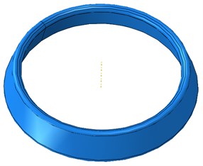
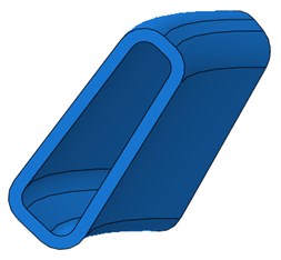
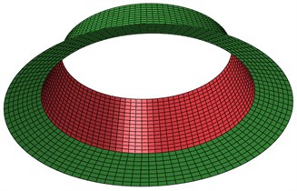
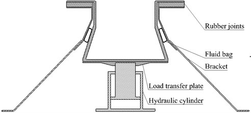
The fluid bag, which is a flexible sealed container, is full of fluid. It is a new kind of nonmetal spring working through the approximate incompressibility of fluid. The diagram of fluid bag is shown in Fig. 1, the outside part is bag cloth, and the inside part is water. The pressure of fluid bag can be adjusted to the predetermined value.
Fig. 1The diagram of fluid bag model
2.2. The application of fluid bag
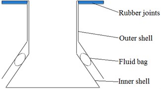
The diagram of a mechanism which requires axial protection is shown in Fig. 2. The inner and outer shell are glued together through the rubber joints. The steel and rubber are vulcanized to the joints, which is similar to the rubber springs for rolling stock [20]. Large axial upward shock loads are imposed on the bottom of inner shell when the mechanism works. However, as for the inner shell, large axial static displacement is not allowed, otherwise the adhesive joints will fail to work. In order to avoid it, a fluid bag which is able to decrease the loads transmitted to the joints, was placed between the inner and outer shell, as is shown in Fig. 3.
Fig. 2The diagram of mechanism
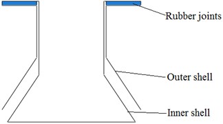
Fig. 3The diagram of mechanism with a fluid bag
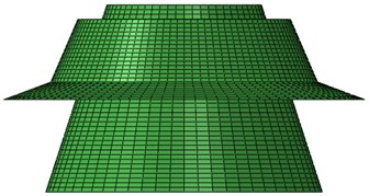
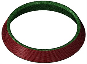
For the purpose of obtaining its axial protection performance, the axial stiffness characteristics of fluid bag will be analyzed alone. The simplified model for analyzing the axial stiffness is shown in Fig. 4. The outer shell was fixed, and the inner shell was adjusted to a predetermined location to be fixed in the axle. The fluid bag pressure was adjusted to a predetermined value. Then the inner shell was set up to be free and large axial loads were applied to its bottom region. The inner and outer shell models are shown in Figs. 5 and 6.
Fig. 4The diagram of simplified model
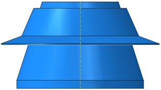
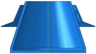
Fig. 5The diagram of inner shell model
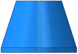
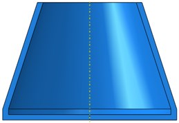
Fig. 6The diagram of outer shell model


While the axial loads are transmitted from the inner shell to rubber joints, the fluid bag are compressed first. Due to the approximate incompressibility of fluid, large loads are generated by the bag under small axial displacement and deformation, avoiding the large static displacement in rubber joints.
3. The analysis of the axial stiffness of fluid bag
3.1. The simulation of fluid bag
In Abaqus, there are a family of elements being able to represent fluid-filled cavities under hydrostatic conditions. The elements provide the coupling between the deformation of fluid-filled structure and the pressure exerted by fluid on the boundary of cavity [21]. When the fluid bag is compressed, the volume and pressure of fluid will change with its deformation. The volume function of fluid is given as:
where is the initial fluid pressure, is the fluid temperature, is the fluid mass. Due to the bag being full of fluid, the fluid volume is always equal to the bag volume. So:
where is the volume of bag cavity.
When the bag deforms, the volume and pressure of fluid will change. When the fluid pressure equals to p, the virtual work contribution due to the fluid pressure is given as:
where is the increment of virtual work and is the virtual work for the bag without the cavity. The negative signs mean that an increase in the bag volume releases energy from the fluid. This indicates a mixed formulation in which the bag displacement and fluid pressure are the two primary variables. The rate of the augmented virtual work expression is shown as:
Eq. (4) can be transformed into:
where indicates the pressure load stiffness, and represents the volume-pressure compliance of fluid.
Since the pressure is the same for all the elements of bag and fluid, the virtual work contribution can also be written as:
Eq. (6) can be transformed into:
where means the virtual strain energy of an element, means the volume a fluid element accounts for in the bag when it is compressed, and means the volume of a fluid element.
Since the temperature is the same for all the elements of fluid, the volume of every fluid element can be expressed as:
where means the mass of an element.
When the external load or fluid pressure changes, so will the shape of bag and fluid. Therefore, the volume a fluid element occupies in the bag may be different from the actual volume of a fluid element. Thus:
However, the total fluid volume is always equal to the bag volume.
To simulate the real mechanical characteristics of fluid bag is to simulate the coupling between the bag and fluid. There are hydrostatic elements being approximate incompressible in Abaqus. These elements can simulate the coupling between the bag deformation and fluid pressure. The fluid mass is related to its density, so the variable can be indicated by . Considering the density, temperature and pressure is respectively uniform, a reference node has been set for all the fluid elements, and the coupling between the reference node and every element has been built. Then the density, temperature and pressure of fluid have been set in the reference node. Thus the real simulation of fluid bag has been completed.
3.2. The finite element model
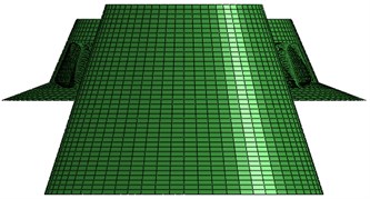
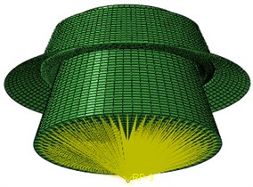
Due to the axial and circumferential size of mechanism being much bigger than its thickness, shell elements were used for the simulation. The S4R finite-strain shell elements were used for the bag, the inner and outer shell. In an attempt to simulate the coupling between the bag and fluid, the fluid elements shared the same nodes with the bag elements. To be specific, the bag elements were duplicated. Then the duplicated elements were changed into F3D4 hydrostatic elements, the element labels being changed and node labels remaining unchanged. The finite element model is shown in Fig. 7.
Fig. 7The finite element model of mechanism
3.3. The simulation of contact
While being compressed, the bag will contact with inner and outer shell. The contact states changes along with the variation of bag shape. However, the rule of this variation is beyond prediction. Therefore, it is necessary to establish real contact pairs. Surface with coarse meshes, a large area and high stiffness are always the master surfaces, and soft surface with a small area and fine meshes are always the slave surfaces [22]. There are two contact pairs in this paper. The first contact pair, the outer surface of inner shell being the master surface and inner diameter surface of bag being the slave surface, is shown in Fig. 8. The second contact pair, the inner surface of outer shell being the master surface and outer diameter surface of bag being the slave surface, is shown in Fig. 9. To ensure an easy convergence for the calculations, tolerance of 0.1 mm has been specified for the two contact pairs.
Fig. 8The master surface and slave surface for first contact pair
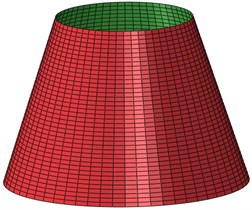
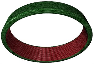
Fig. 9The master surface and slave surface for second contact pair
3.4. The boundary conditions and material properties
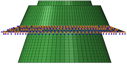
According to chapter 2.2, the outer shell is fixed. For the purpose of axial loads being imposed easily, the continuous distributing coupling was established between the coordinate origin and the bottom surface of inner shell, making the loads imposed on the coordinate origin distribute on the bottom surface of inner shell. The boundary conditions and load coupling are shown in Fig. 10.
Fig. 10The diagram of boundary conditions and load coupling
The material of inner and outer shell is high-strength steel. The bag material is rubber fiber, and the bag is full of water. The equivalent elastic modulus, Poisson’s ratio and density are given in Table 1.
Table 1The material properties of model
Material | Density (kN/mm3) | Elastic modulus (MPa) | Possion’s ratio | Bulk modulus (MPa) |
High-strength steel | 7.8×10⁻⁹ | 2.1×10⁵ | 0.3 | |
Rubber fiber | 1.4×10⁻⁹ | 7×10³ | 0.3 | |
Water | 2200 |
3.5. The experimental verification of axial stiffness characteristics
Due to the fluid bag providing axial protection for rubber joints, the whole stiffness of fluid bag and joints were measured in experiments. Then the stiffness of fluid bag could be derived from the stiffness of joints measured in advance. The inner shell would be restricted by the joints while moving down in the axle. Therefore, its position does not need to be adjusted while the bag are being filled with fluid.
3.5.1. The introduction of experiment
The schematic is shown in Fig. 11, where the inner and outer shell are connected by the rubber joints as displayed. The fluid bag lies between the inner and outer shell. Four brackets, being made of steel, are bolted with the outer shell and pinned to the ground uniformly. A piece of load transfer plate is attached and bolted to the inner shell, and is connected to the hydraulic cylinder.
Fig. 11The experimental schematic diagram
A pressure sensor is established at the orifice of the fluid bag for the purpose of measuring the pressure inside the fluid bag. Four displacement sensors are placed on the edge of the bottom of the inner shell, which will offer an average displacement value for the experiment. The pressure sensor, displacement sensor, dynamic testing instrument and hydraulic cylinder is respectively shown in Fig. 12 to Fig. 15.
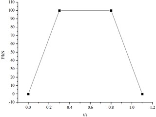
The form of load in the experiment is shown in Fig. 16.
Fig. 12The pressure sensor
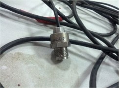
Fig. 13The displacement sensor
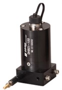
Fig. 14The dynamic testing instrument

Fig. 15The hydraulic cylinder
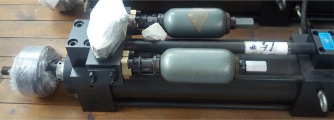
Fig. 16The curve of load varying with time
The experiment procedures are listed below.
Step 1, the stiffness of the rubber joints without the fluid bag was measured. The load was applied as required, and the displacement of the edge of the bottom of the inner shell along the axial direction was measured.
Step 2, the fluid bag was placed between the inner and outer shell, and was pressurized to 1.5 MPa. The air in the bag being exhausted as far as possible, the load was applied according to the requirement, and the displacement of the edge of the bottom of the inner shell along the axis direction as well as the pressure in the fluid bag was tested.
Step 3, the initial pressure of the bag was set to 2.0 MPa, then other procedures in Step 2 were repeated.
Step 4, according to the data from last three steps, the displacement-load curve and pressure-load curve were formed. Afterwards, the least square method was used to form the linear fitting chart and the slopes of the lines were acquired.
Step 5, from Step 4 the axial stiffness of the rubber joints and the axial stiffness of the fluid bag together with the rubber joint were acquired.
3.5.2. The comparison between simulation and experiment results
When the initial bag pressure is 1.5 MPa, the simulation and experiment results are shown in Fig. 17 and Fig. 18.
When the initial bag pressure is 2.0 MPa, the simulation and experiment results are shown in Fig. 19 and Fig. 20.
Fig. 17The diagram of whole axial stiffness of simulations and experiments
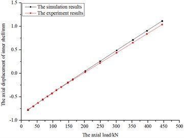
Fig. 18The diagram of bag pressure of simulations and experiments
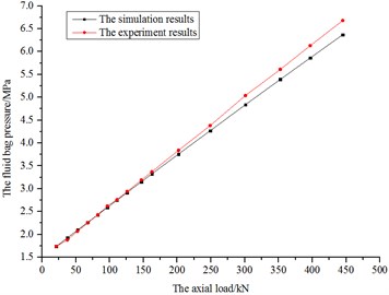
Fig. 19The diagram of whole axial stiffness of simulations and experiments
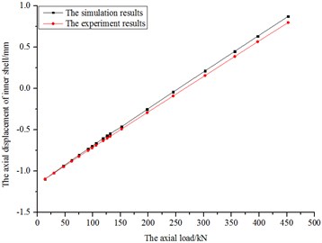
Fig. 20The diagram of bag pressure of simulations and experiments
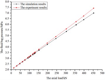
According to Fig. 17 to Fig. 20, the curves of axial stiffness and pressure variations have good linearity. The difference of results between the simulations and experiments is small, proving the correctness of simulations.
Table 2The whole axial stiffness under different initial bag pressures
The bag pressure / MPa | The axial stiffness of inner shell (kN/mm) | |
The simulation result | The experimental result | |
1.5 | 224.3 | 234.7 |
2.0 | 222.8 | 231.6 |
As for the rubber joints, the elastic modulus of steel is 210000 MPa, and the equivalent modulus of rubber is 1.25 MPa. The measured axial stiffness of rubber joints is 74.2 kN/mm. Therefore, the measured axial stiffness of fluid bag is 160.5 kN/mm under 1.5 MPa initial pressure, and the value would be 157.4 kN/mm under 2.0 MPa initial pressure.
According to Fig. 18 and Fig. 20, the fluid bag is compressed by the inner shell with the increasing axial load. Due to the bag being full of approximately incompressible fluid, the bag pressure increases rapidly during the progress. Most of the loads on the inner shell could be transmitted to outer shell through the fluid bag, providing axial protection for the rubber joints. And the bag pressure variations of simulations and experiments are very similar, which demonstrates that the simulations hold water.
4. The factors affecting the axial stiffness characteristics
The fluid bag was positioned between the inner and outer shell, and the axial displacement of inner shell was adjusted to –0.35 mm. Then the inner shell was fixed. The temperature of reference node was set to 20°C, and the fluid density was 1×10⁻⁹ kN/mm3. Then the bag got filled with fluid: the bag pressure being set to , the pressure was calculated when the fluid bag was in balance. If had not reached the initial working pressure predetermined, would be adjusted until met it. Then all the constraints of inner shell got removed. Meanwhile, the axial load was imposed on the bottom of inner shell, analyzing the axial stiffness characteristics of fluid bag.
According to the model in Chapter 2, the axial stiffness of fluid bag was calculated. When the initial pressure is 2.5 MPa and load is 250 kN, the results are shown in Fig. 21 and Fig. 22.
Fig. 21The stress nephogram of mechanism when the load is 250 kN
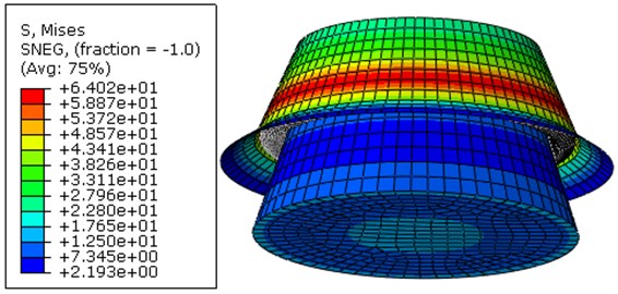
Fig. 22The axial displacement nephogram of mechanism when the load is 250 kN
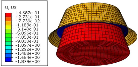
According to Fig. 21 and Fig. 22, the stress and axial displacement nephogram are evenly distributed in the circumferential. According to Fig. 22, the fluid bag moves downward when the inner shell moves upward along the axle.
4.1. The axial stiffness of fluid bag under different initial pressures
The results are displayed in Fig. 23 to Fig. 27 when the initial pressure is respectively 1.5 MPa, 2.0 MPa, 2.5 MPa, 3.0 MPa and 3.5 MPa.
Fig. 23The diagram of axial displacement and load of inner shell
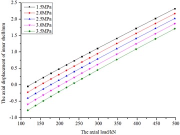
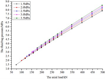
Fig. 24The diagram of bag pressure and load
According to Fig. 23, the axial stiffness of fluid bag remains basically unchanged with load increasing when an initial pressure is exerted. The axial stiffness remains basically unchanged when the initial pressure turned from 1.5 MPa to 3.5 MPa. According to the calculations, while the initial pressure varies from 1.5 to 3.5 MPa, the corresponding stiffness are 160.93, 158.95, 156.91, 154.98 and 153.12 kN/mm, which are extremely close to the experimental results.
According to Fig. 24, the initial loads are different, owing to the fluid bag having different balanced loads when different initial pressures are exerted. The bag pressure increases along with load, and the pressure variation tendency has tiny nonlinearity. For example, when the load is 177.28 kN and initial pressure is respectively 1.5 to 3.5 MPa, the corresponding bag pressure is 3.23, 3.30, 3.38, 3.44 and 3.50 MPa, and the pressure difference of adjacent curves are respectively 0.079, 0.072, 0.067 and 0.058 MPa. When the load increases to 497.28 kN, the corresponding bag pressures are 7.91, 8.09, 8.27, 8.42 and 8.56 MPa, and the pressure difference of adjacent curves are respectively 0.179, 0.172, 0.156 and 0.141 MPa. The pressure difference of adjacent curves increases with load when different initial pressures are exerted.
Fig. 25The diagram of inner contact area and load
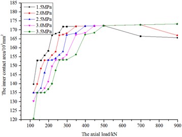
Fig. 26The diagram of outer contact area and load
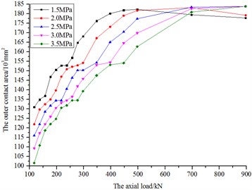
In Fig. 25 and Fig. 26, the inner contact area means the contact area between inner shell and fluid bag, and the outer contact area means the area between outer shell and fluid bag. According to the figures, the inner and outer contact area both increase along with load, after reaching their respective maximum values, they are likely to almost remain unchanged under different initial pressures, except for 1.5 and 2.0 MPa. Owing to being relatively soft, the bag is gradually compressed by the increasing load, making the contact area gradually expand. Due to being not able to be compressed unlimitedly, the contact area will remain basically unchanged after reaching their peak figures. While the initial pressure is respectively 1.5 and 2.0 MPa, the contact area shrinks with load after reaching their peak figures. According to Fig. 22, due to the fluid bag moving downward with load, the low part of bag would no longer contact with the inner and outer shell after the contact area reaching peak figures, which eventually leads to the reduction of the area of contact.
The corresponding contact area decreases with the initial pressure. The higher initial pressure, as well as the large amount of fluid contained by the bag, is likely to reduce the initial contact area. However, when the contact area reaches peak figures, the corresponding load would increase with initial pressure. It can be inferred that the higher the initial pressure is, the stronger the bag’s ability to resist deformation is.
Fig. 27The diagram of bag volume and load
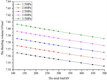
According to Fig. 27, the bag volume decreases with load, and the variation tendency remains basically unchanged under different initial pressures.
4.2. The axial stiffness of fluid bag under different material properties
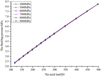
The initial pressure of fluid bag is 2.5 MPa, and the fluid bulk modulus is 2200 MPa. The results are shown in Fig. 28 and Fig. 29 when the elastic modulus of bag is respectively 4000, 5000, 6000, 7000, 8000 and 9000 MPa.
Fig. 28The diagram of axial displacement and load of inner shell
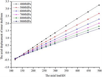
Fig. 29The diagram of bag pressure and load
According to Fig. 28, the axial stiffness of fluid bag is evidently different under different elastic modulus. The axial stiffness increases with elastic modulus, but the trend of rising grows weaker afterwards. For example, when the elastic modulus of bag varies from 4000 to 9000 MPa, the corresponding stiffness are 101.84, 121.74, 140.03, 156.91, 172.55 and 187.09 kN/mm, and the stiffness differences between the adjacent curves are respectively 19.9, 18.29, 16.88, 15.64 and 14.54 kN/mm.
According to Fig. 29, all the curves almost coincide with one another, indicating that the difference of elastic modulus basically has no effects on the bag pressure variation.
4.3. The axial stiffness of fluid bag under different fluid bulk modulus
The initial pressure of fluid bag is 2.5 MPa, and the elastic modulus of bag is 7000 MPa. The results are shown in Fig. 30 and Fig. 31 when the fluid bulk modulus is respectively 200, 400, 600, 1000, 1400, 1600, 1800, 2000, 2200 and 2400 MPa.
Fig. 30The diagram of axial displacement and load of inner shell
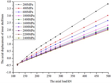
Fig. 31The diagram of the pressure and load
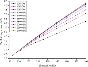
According to Fig. 30 and Fig. 31, the axial stiffness and bag pressure increase with load, but the increasing trends are becoming weaker.
The axial stiffness and pressure variation of fluid bag have bad linearity when the fluid bulk modulus is small. It is indicated that the fluid is easy to be compressed under small bulk modulus, making the bag have relatively large deformation. However, with the fluid bulk modulus increasing gradually, the fluid becomes difficult to be compressed, making the deformation progress harder to occur on the bag. Thus the curves have relatively good linearity.
4.4. The finite element analysis of fluid bag for axial protection
According to Chapter 2.2, the inner and outer shell are glued together through the rubber joints. And the inner shell will have a big impact upward in the axle when the mechanism works. If the stress in the rubber joints is too large, it may lead to the mechanism failing to work. Therefore, it is necessary to decrease the stress in the joints.
Fig. 32The finite element model of mechanism
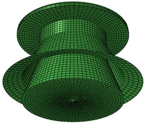
Fig. 33The finite element model of mechanism with a fluid bag
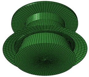
In order to obtain the bag’s ability to decrease the stress, a simplified shock model has been established. Considering the exactitude and efficiency in calculation, the rubber joints are simplified as a rubber pad. Due to the focus of research being the bag’s ability to decrease the stress, the modeling of adherend layer is ignored. The exact model is shown in Fig. 32. It is assumed that the outer shell is stationary while the load is transmitted upward. Thus the outer shell is fixed. The finite element model of mechanism with a fluid bag is shown in Fig. 33. The joints, inner and outer shell are joined together with tie constraints. The material properties are shown in Table 1, and the boundary conditions are shown in Fig. 10.
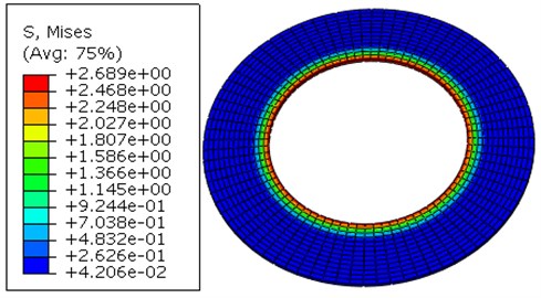
When the load is 250 kN, the stress distribution between the joints and inner shell is shown in Fig. 34 to Fig. 37.
According to Fig. 34 to Fig. 37, the stress distribution trends are basically the same whether mechanism has a bag or not. When it comes down to the mechanism without a bag, the maximum stress between the bag and inner shell is 5.525 MPa, and the value between the bag and outer shell is 6.066 MPa. While the mechanism has a bag, the value between the bag and inner shell becomes 2.449 MPa, and the value between the bag and outer shell becomes 2.689 MPa. It is indicated that the bag can decrease the stress in the joints effectively, having a good performance for axial protection.
Fig. 34The diagram of stress between the joints and inner shell without the fluid bag
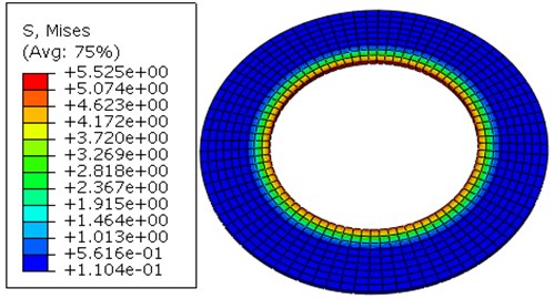
Fig. 35The diagram of stress between the joints and outer shell without the fluid bag
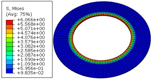
Fig. 36The diagram of stress between the joints and inner shell with a fluid bag
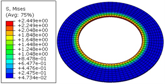
Fig. 37The diagram of stress between the joints and outer shell with a fluid bag
5. Conclusions
1) The fluid bag is designed for axial protection under small displacement and deformation. The hydrostatic elements are used to simulate the incompressible fluid, and the hydrostatic theory is applied to simulate the coupling between the bag and fluid. The axial stiffness and pressure variation of bag both has good linearity. The disparity between the simulations and experimental results seems to be quite small, proving the accuracy of simulations.
2) The effects of initial pressure on the fluid bag have been discussed. When the initial pressure varies from 1.5 MPa to 3.5 MPa, the axial stiffness and pressure variation of bag would basically maintain their original values.
3) The effects of material properties on the fluid bag are discussed. Despite having no effects on the pressure variation, the elastic modulus of bag appears to be one of the crucial factors affecting its axial stiffness characteristics. The axial stiffness of bag increases with its elastic modulus.
4) The effects of fluid bulk modulus on the fluid bag are discussed. The bulk modulus is another crucial factor affecting the axial stiffness. The nonlinearity of axial stiffness and pressure variation curves gradually becomes weak with the bulk modulus. The axial stiffness of bag increases with the fluid bulk modulus, and the slope of pressure varying with load increases with the fluid bulk modulus.
5) The effects of fluid bag on a shock mechanism are discussed. The fluid bag can effectively decreases the stress in the rubber joints, having a good performance for axial protection.
References
-
Chew A., Brewster B., Olsen I., et al. Developments in nEXT turbomolecular pumps based on compact metal spring damping. Vacuum, Vol. 85, Issue 12, 2011, p. 1156-1160.
-
Cho J. R., Moon S. J., Moon Y. H., et al. Finite element investigation on spring-back characteristics in sheet metal U-bending process. Journal of Materials Processing Technology, Vol. 141, Issue 1, 2003, p. 109-116.
-
Chan W. M., Chew H. I., Lee H. P., et al. Finite element analysis of spring-back of V-bending sheet metal forming process. Journal of Materials Processing Technology, Vol. 148, Issue 1, 2004, p. 15-24.
-
Berg M. A non-linear rubber spring model for rail vehicle dynamics analysis. Vehicle System Dynamics, Vol. 30, Issues 3-4, 1998, p. 197-212.
-
Wang L. R., Lu Z. H., Hagiwara I. Finite element simulation of the static characteristics of a vehicle rubber mount. Proceedings of the Institution of Mechanical Engineers, Part D: Journal of Automobile Engineering, Vol. 216, Issue 12, 2002, p. 965-973.
-
Luo R. K., Wu W. X. Fatigue failure analysis of anti-vibration rubber spring. Engineering Failure Analysis, Vol. 13, Issue 1, 2006, p. 110-116.
-
Toyofuku K., Yamada C., Kagawa T., et al. Study on dynamic characteristic analysis of air spring with auxiliary chamber. JSAE Review, Vol. 20, Issue 3, 1999, p. 349-355.
-
Xiao J., Kulakowski B. T. Sliding model control of active suspension for transit buses based on a novel air-spring model. American Control Conference, 2003, p. 3768-3773.
-
Presthus M. Derivation of air spring model parameters for train simulation. Master’s Thesis, Department of applied physics and mechanical engineering, Division of fluid mechanics, LULEA University, 2002.
-
Tsai C. L., Guan Y. L., Ohanehi D. C., et al. Analysis of cohesive failure in adhesively bonded joints with the SSPH meshless method. International Journal of Adhesion and Adhesives, Vol. 51, 2014, p. 67-80.
-
Dorn L., Liu W. The stress state and failure properties of adhesive-bonded plastic/metal joints. International Journal of Adhesion and Adhesives, Vol. 13, Issue 1, 1993, p. 21-31.
-
Gent A. N., Yeoh O. H. Failure loads for model adhesive joints subjected to tension, compression or torsion. Journal of Materials Science, Vol. 17, Issue 6, 1982, p. 1713-1722.
-
Giner E., Sukumar N., Tarancon J. E., et al. An Abaqus implementation of the extended finite element theory. Engineering Fracture Mechanics, Vol. 76, Issue 3, 2009, p. 347-368.
-
Chang B., Shi Y., Lu L. Studies on the stress distribution and fatigue behavior of weld-bonded lap shear joints. Journal of Materials Processing Technology, Vol. 108, Issue 3, 2001, p. 307-313.
-
Al-Samhan A., Darwish S. M. H. Finite element modeling of weld-bonded joints. Journal of Materials Processing Technology, Vol. 142, Issue 3, 2003, p. 587-598.
-
Goncalves V. M., Martins P. A. F. Static and fatigue performance of weld-bonded stainless steel joints. Materials and Manufacturing Processes, Vol. 21, Issue 8, 2006, p. 774-778.
-
Wakui S. Incline compensation control using an air-spring type active isolated apparatus. Precision Engineering, Vol. 27, Issue 2, 2003, p. 170-174.
-
Shimozawa K., Tohtake T. An air spring model wit non-linear damping for vertical motion. Quaterly Report of RTRI, Vol. 49, Issue 4, 2008, p. 209-214.
-
Wang J. S., Zhu S. H. Linearized model for dynamic stiffness of air spring with auxiliary chamber. Journal of Vibration and Shock, Vol. 28, Issue 2, 2009, p. 72-76, (in Chinese).
-
Lan Qing-qun, Wu Ping-bo Static and dynamic analysis of rubber spring for rolling stock. Machinery Design and Manufacture, Vol. 11, 2008, p. 43-45, (in Chinese).
-
Abaqus 6.10 Online Documentation. Abaqus Theory Manual, 4-28-2010.
-
Gong Longying On the use of Abaqus for analyzing the problem of contacts. China Coal, Vol. 35, Issue 7, 2009, p. 66-68, (in Chinese).
About this article
