Abstract
Conventional modal testing requires a known excitation force in order to extract the modal properties. One particular challenge using this technique is that it can be experimentally complex because of the need for artificial excitation and it also does not represent actual operational condition. The present study had successfully applied a real time modal testing technique for cantilevered flexible composite plate which is exposed to subsonic flow in an open-looped wind tunnel. The technique only employed two sensors which consist of a single contactless sensing system via a laser vibrometer and an accelerometer as reference. The measured response data was extracted using Frequency Domain Decomposition (FDD) technique. The modal testing was conducted at various air speed and the effects on modal properties are investigated. Conventional modal testing was performed to establish the modal properties. With increasing air speed, the bending modes appeared unaffected, however the frequencies of the torsional modes showed significant increase.
1. Introduction
Over recent decades, modal testing and analysis has been widely applied for aerospace structures, mechanical and civil engineering in determining and optimizing the dynamic characteristics of the structures [1, 2]. In aerospace applications, interactions of airflow with aircraft structures, better known as aeroelasiticity, can result in undesirable deformations that can be destructive in nature and compromise its structural stability. A particular dynamic instability, flutter, resulted from coupled structural modes of the vibrating system. Therefore prior knowledge of the dynamic properties are necessary for validating and improving its structural dynamic model as part of the flutter clearance process and these are usually achieved via ground vibration testing through hammer or shaker testing, depending on the size and complexity of the structure.
Experimental modal analysis (EMA) has become an establish method in determining the natural modes in the last three decades [3]. It involved artificially exciting the structure and measuring the response. Frequency Response Functions (FRFs) which is the ratio of the response (output) signal over the excitation (input) signal is calculated and the frequency peak amplitudes are identified as possible modes. However, traditional EMA has limitation whereby FRFs would be very difficult or even impossible to be measured within the operational condition. In this case, Operational Modal Analysis (OMA) or also named as ambient or output-only analysis is a suitable technique to be applied. It does not require special boundary conditions, measurements are in-situ, uses natural excitation and can be performed simultaneously with other testing. The objective of OMA is to identify the modal properties of a system which are the frequency resonances, damping and mode shapes by using only output measured responses and without knowledge of the inputs. In aerospace industry, to predict flutter occurrence, wind tunnel testing is a crucial experiment and performed on a new or modified aircraft before the first flight [4]. Due to this matter, OMA would be very attractive tool since in wind tunnel condition, the airflow turbulence can be used to provide the necessary excitation required for OMA testing.
Since early 1990’s, OMA has drawn great attention in many engineering fields such as mechanical, civil and aerospace community itself [5, 6]. Apart from aerospace, other applications include bridges, roads, buildings as well as automotive such as cars and engines. In bridges, the vibration modes induced by traffic and wind are of interest [7], while in automotive, the resonances from engine run-up as well as investigation of on-the-road body vibrations in the development of new cars are among the objectives of conducting OMA [8].
To ensure good modal data is attainable, three specific requirements for the excitation must be fulfilled which are the power spectra of the input forces are broadband and smooth; the input forces are uncorrelated; and distributed over entire structure [9]. In a wind turbine example [9], airflow turbulence appeared to fulfill these requirements however, the presence of aeroelastic effects, presence of rotational components in the excitation forces and time varying nature of the flow contradicted these requirements. In spite of that, efforts on applying OMA for wind tunnel testing are carried out for example in references 10 and 11. However, these are lacking on the contribution of the effect of airspeed in subsonic condition.
In this present paper, OMA techniques are demonstrated on a cantilevered composite thin plate subject to random tapping excitation as well as excitation from the airflow in wind tunnel environment. Therefore, the tested models and experimental setups of OMA system for wind tunnel environment, procedures and results obtained via EMA and OMA will be discussed in the following sections.
2. Theoretical background
2.1. Aeroelastic effects
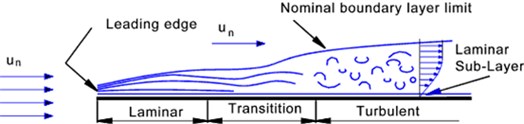
The Re number ranged from 2.2 X 10⁴ to 5.1 X 10⁴ for this testing. In this range the boundary layer flow is laminar and it is very difficult to cause transition to turbulent flow [12]. To create air turbulence, the angle of attack was set to zero. Leading edge separation may occur at low angle of attack leading to a boundary layer separation as seen in Fig. 1.
Fig. 1Boundary layer separation over a flat plate
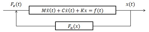
Configuration-wise, cantilevered problems are more difficult to tackle due to the complication caused by downstream wake effects [14]. In addition, aeroelastic interactions between the plate and air surrounding enhance the surrounding turbulence surrounding the thin plate. This aeroelastic effect can be described in the feedback diagram shown in Fig. 2, where , and are the mass, damping and stiffness matrices, is the structural deformation and represents the aerodynamic forces applied on the structure. can be divided into two parts; , the aerodynamic force induced by the structural deformation and , the external force acting on it. Since depend on the structural deformation, the relationship can be predicted as an aerodynamic feedback. If flutter occurs, then damping is zero and the equation of motion reduces to a self-excited vibration.
Fig. 2Aeroelastic feedback diagram
2.2. Analysis
The basis of modal analysis is the so called system equation of Fourier Transform [1] given by equation:
in frequency domain, where contains the set of Frequency Response Functions (FRFs) of the system. In EMA, where both input and output are known, the FRFs can directly be calculated and used for model extraction. The Frequency Domain Decomposition (FDD) is an extension of the classical frequency domain approach or more often called the Peak-picking Technique. It has been introduced by Brincker et al. [15] in 2000. Since is not known in OMA, though, further mathematics and assumptions are needed. Equation (1) can be enhanced onto power spectral densities (PSD) [15]. The relationship between the input and output can be written in the following form:
where is the input PSD matrix. is the output PSD matrix, and is the FRF matrix and and denote complex conjugate and transpose, respectively. Applying the Fourier transform in Eq. (1) gives:
where is the spectrum matrix of the modal coordinates. With:
This matrix represents mode shapes. The FDD technique is based upon the SVD of the Hermetian response spectrum matrix at each frequency and for each measurement (data set):
where is the singular value diagonal matrix and is the orthogonal matrix of the singular vectors. The singular vectors the columns in are orthogonal to each. The simple peak-picking technique is applied in the first singular line to obtain frequency and associated mode shapes. But this technique has no damping ratios estimation.
3. Methodology
3.1. Composite plate
The composite plate is fabricated from woven carbon/kevlar fiber with epoxy resin. The fabrication process is via vacuum bagging and the stacking sequence was [0/90]3. The geometry is of low aspect-ratio wing with dimensions of 100 mm by 500 mm and thickness of 2.4 mm giving thickness-to-chord ratio of 2.4 %. It weighed at 45 grams which required a miniature accelerometer to avoid mass loading effect. Fig. 3 showed the fabricated composite plate.
3.2. Finite element modelling
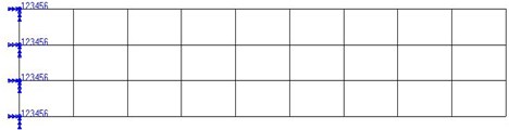
Prior to experimental work, modal analysis is conducted through finite element modelling to gain valuable insights of the modal parameters. In modal analysis, only the structural model are required and the effects of air flow is not considered here. The finite element model of the composite plate is modelled using 30 CQUAD4 shell elements (see Fig. 4). The material properties are obtained via ASTM D3039 and the element properties are defined as quasi-isotropic. Translational and rotational displacements at the root nodes are defined as zero to simulate the fixed-end boundary conditions.
Fig. 3Composite thin plate model

Fig. 4Finite element model
3.3. Experimental modal testing
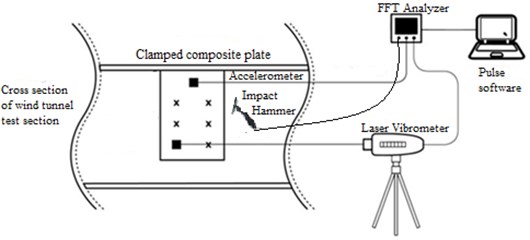
The technique Single Input Single Output (SISO) whereby one miniature hammer provides the excitation and one fixed miniature accelerometer as reference is used. The modal response is measured via a uniaxial accelerometer and also laser vibrometer. The measured FRFs are then post-processed using ME’scope software to extract the modal parameters such as modal frequencies, damping ratio and mode shapes. All measurements utilized Brüel & Kjær PULSE Fast Fourier Transform (FFT) analyzer type 3560c. The composite plate is mounted in the wind tunnel, clamped at the top as shown in Fig. 5. The procedure involved exciting the plate structure on each of the 30 points using the impact hammer in the direction of measurement. The process is repeated three times and the coherence of the averaged data are monitored to ensure good quality data are obtained. For all measurements, coherence of 0.8 is considered reasonable acceptance criteria since composite structures are highly damped.
Fig. 5Experimental modal testing set up
3.4. Operational modal testing
Contrary to EMA, this technique requires similar setup to EMA (see Fig. 5) except in terms of the excitation which is provided by real operational condition. In this case, the technique was demonstrated using two types of excitation, i.e. continuous random tapping and air flow turbulence in wind tunnel. Data were recorded using the same response transducers whereby the accelerometer was used as reference whereas the laser vibrometer was roved to measure at dedicated points on the plate. For random tapping, two fingers are used to continuously tap on the composite plate models to avoid signal loss or drop-outs in signals. Meanwhile, for airflow or wind-on excitation technique, the procedure is to increase the airspeed and dwell at certain speed and then the measurement was taken for a specific time interval. In OMA, the correlation time for a certain mode can be defined as . This means that the data segments should at least have that length to reasonably avoid the influence of leakage. The minimum duration of the continuous measurement therefore should be where is the lowest natural frequency and is modal damping [15]. For the current work, time interval calculated based on first mode obtained via EMA was 56 seconds. To gauge the effect of airspeed, the dwell speed was ranged from rotor speed of 0 m/s up to speed of flutter onset which physically was observed to occur at 7.3 m/s. According to Tcherniak et al. [9], a constant speed does not result in broadband frequency content, however, due to the aeroelastic effects described in the previous section, it was believed that this will contribute to significant air turbulence and provide the necessary stochastic input required.
3.5. Wind tunnel testing
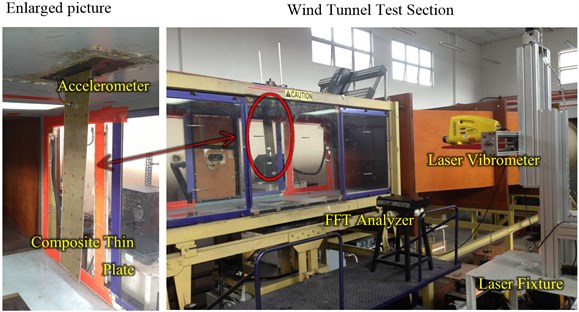
The present testing was performed in an open-looped subsonic wind tunnel with 1 m by 1 m test section. The wind tunnel has a maximum flow velocity of 40 m/s and turbulence level is low depending on range of operating test-section velocities. The composite plate was fixed at the top of the test section and measurement points marked with reflective tape for accurate laser detection. A jig mounting for the vibrometer was fabricated that allow it to automatically rove horizontally and vertically over the plate surface during measurement (see Fig. 6). The reference accelerometer is attached at one of the measurement points near the root of the plate to reduce the disturbance due to the wiring attachment on the plate.
Fig. 6Wind tunnel test setup
4. Results and discussions
4.1. FE result
The first five natural frequencies and the corresponding mode shapes of the model are extracted using MSC/NASTRAN are shown in Table 1. It can be seen that the first five modes of the thin plate are in the frequency range of 1.7 Hz to 54.0 Hz. With the FE results, the frequency range was approximated up to 100 Hz and the mode shapes predicted helped to determine the placement for the transducer.
Table 1Natural frequencies and mode shapes obtained from FE
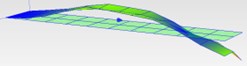
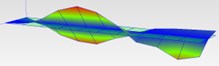
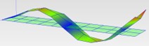
 1.7 Hz (1st Bending) | 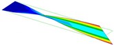 9.6 Hz (1st Torsion) |  10.7 Hz (2nd Bending) | 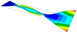 30.1 Hz (2nd Torsion) | 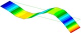 54.0 Hz (3rd Bending) |
4.2. EMA Result
Typical curve fitted FRFs obtained from accelerometer and laser scanning testing with impact hammer excitation is shown in Fig. 7 and 8. Comparing the FRFs measured using accelerometer and laser vibrometer showed strong agreement between the two results which meant that the effect of mass for a single accelerometer is negligible in this instance except for mode 1 where there is a drop in coherence. This could be due to the sensitivity of the miniature accelerometer that may not be able to capture low frequency mode. One of the instrumentation constraints with EMA is the effect of the transducer mass on the structure [16, 17]. With the influence of the transducer mass, it will introduce larger inertia effect which caused spatial complexity of the modes and this justifies the need for optical sensor. This EMA results will be compared with OMA results for mode frequencies and mode shapes comparison. Modal parameters were derived from FRFs and tabulated in Table 2 for different response measured by accelerometer and laser vibrometer.
Fig. 7FRF plot after curve fitting measured via accelerometer. M#1 1Z:4Z Frequency Response H1 (accelerometer, hammer) – STS Measurement 1, Input: STS FFT Analyzer (Log Magnitude)
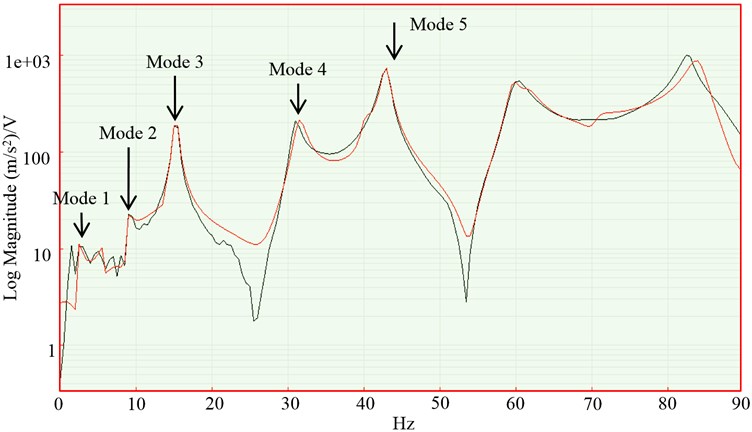
Fig. 8FRF plot after curve fitting measured via laser vibrometer. M#1 1Z:4Z Frequency Response H1 (laser, hammer) – STS Measurement 1, Input: STS FFT Analyzer (Log Magnitude)
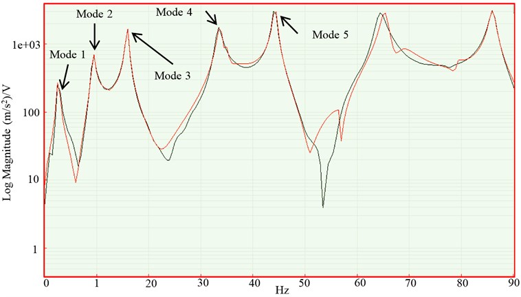
Table 2Mode frequencies and damping ratios obtained from impact test
Mode Type | Natural frequency, (Hz) | Error (%) | Modal damping, (%) | ||
Accelerometer | Laser Vibrometer | Accelerometer | Laser Vibrometer | ||
1B | 2.53 | 2.66 | 5.14 | 7.99 | 6.69 |
1T | 8.93 | 9.20 | 3.02 | 3.56 | 2.64 |
2B | 15.20 | 15.90 | 4.61 | 1.60 | 1.51 |
2T | 31.50 | 33.70 | 6.98 | 2.27 | 1.37 |
3B | 42.90 | 44.30 | 3.26 | 1.24 | 0.78 |
4.3. OMA result
Example of time histories of the measured response is shown in Fig. 9 and must display time decay behaviour. For wind-on excitation, it was found that valid time histories are obtained within the range of 3.2 m/s to 6.3 m/s (5 to 8 Hz rotational speed of drive motor). Therefore, measurements were taken at 3.2, 5.7 and 6.3 m/s. Higher than this (approximately 9 Hz), the thin plate starts to undergo limit cycle oscillation flutter. The first 5 natural frequencies was tabulated in Table 3 and showed that while the bending modes are in excellent agreement between the random tapping and wind-on techniques, the torsional modes are not.
Fig. 9Time histories of the measured response
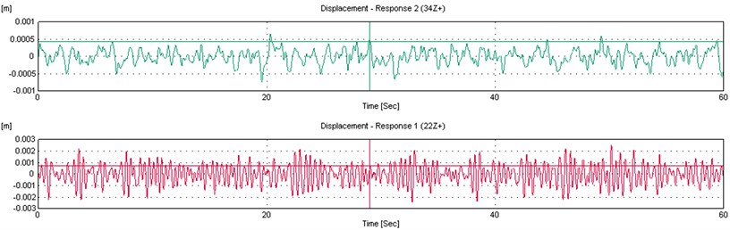
Table 3OMA results
Mode Type | Random tapping | Wind-on excitation | ||
Natural frequency, (Hz) | Natural frequency, (Hz) | |||
Airflow speed (m/s) | ||||
3.2 | 5.7 | 6.3 | ||
1st Bending | 2.75 | 2.50 | 2.5 | 2.63 |
1st Torsion | 10.50 | 7.25 | 12.38 | 11.50 |
2nd Bending | 15.75 | 15.63 | 16.13 | 15.88 |
2nd Torsion | 34.50 | 29.63 | 37.25 | 38.16 |
3rd Bending | 44.25 | 44.13 | 44.00 | 44.00 |
The identification of the modal frequencies from random tapping and wind-on excitations were presented in typical FDD plots as shown in Fig. 10 and 11. The FDD plot for random tapping is smoother and displayed more prominent peaks corresponding to the natural frequencies of the plate. In contrast, the FDD plot for wind-on excitation displayed more noise and less prominent peaks. To ascertain that peaks do represent the modal peaks, the mode shapes at those peaks are to be examined and if it is complex, then that particular peak are ruled out. However, in this case, predicting the mode shapes prior to testing via finite element analysis is necessary. For heavier structures, the quality of the FDD can be improved by conducting single testing as opposed to roving test through the use of multiple transducers.
Fig. 10FDD for random tapping
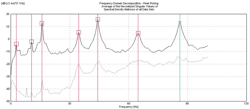
Fig. 11Example of FDD for wind-on

4.4. Effects of airspeed on natural frequency
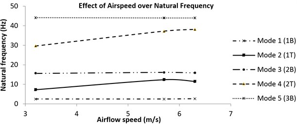
From Table 3, it was observed that the modal frequencies are affected by the magnitude of the wind-on excitations. The airflow give rise to the plate’s motion and in return, the plate’s motion will create or change the unsteady pressure distribution to the surrounding flow and vice versa in such way that the effects are increased with increasing speed. In the FDD plots for different airspeeds (not given in this paper), the shift in the peaks are noted corresponding to the effects of the airspeed. The trend of the frequency with airspeed is further described in Fig. 12.
If the airspeed is zero, the frequency corresponds to the natural frequency of the plate. There is no significant trend observed in the bending modes except when the speed approaches the critical flutter speed, slight decrease or increase of the frequencies are observed in 1st and 2nd bending modes, indicating their contribution to flutter. Frequency of third bending mode remains unchanged indicating the lack of contribution to flutter. For the torsional modes (1T and 2T), the frequencies significantly increases with airspeed. The behaviour of the frequencies of these modes are as expected, whereby flutter is defined as coupling of bending and torsional modes. The coupling is indicated by the merging of the two frequencies in which one is diverging and one is decaying.
Fig. 12Trend of the frequency with airspeed
4.5. Structural mode shapes
From the estimation of the structural mode shapes, the thin plate model that was excited in airflow was compared on the structural mode shapes produced via EMA as shown in Table 4. Except for mode 1 that displayed a complex mode, the rest showed good correlation. Although the FDD plot (Fig. 11) displayed a significant peak at 1st bending, the mode shape was discovered to be complex. This again is due to the sensitivity of the miniature accelerometer used as the reference in the test setup.
Table 4Structural mode shapes produced via EMA and OMA
EMA | OMA (6.3 m/s) | |
Mode shapes |  2.66 Hz (1B) |  2.63 (Complex mode) |
 12.2 Hz (2T) |  11.50 (1T) | |
 15.9 Hz (2B) | 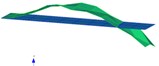 15.88 (2B) | |
 33.7 Hz (2T) | 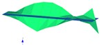 38.16 (2T) | |
 44.3 Hz (3B) | 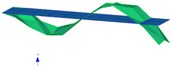 44.00 (3B) |
5. Conclusions
Performing a modal test on a highly damped material such as composite is a challenging task. The difficulty is not in measuring the response but in exciting the structure. From the results presented and discussed, it was demonstrated that the implementations of the OMA in determining the modal frequencies and mode shapes could be achieved via random tapping and wind-on excitation techniques with minimum transducers. The result of this modal data was then compared with more establish technique such as EMA. It was found that, the frequencies of the modes are affected by the airflow. This indicates that the modal properties obtained via conventional EMA testing are not representative of the actual behavior when exposed in airflow. Further works should be carried out to evaluate how these will affect flutter predictions.
References
-
Jimin He, Zhi-Fang Fu Modal Analysis. Butterworth-Heinemann. 2001.
-
W.T. Thomson Theory of Vibration with Applications. George Allen & Unwin, 1981.
-
Peeters B., Leurs W., Auweraer H. van Der, Deblauwe F. 10 Years Of Industrial Operational Modal Analysis: Evolution In Technology And Applications Technology evolution, 2006.
-
Peeters B., Climent H., Diego R. De, Alba J. De, Ahlquist J. R., Carreño J. M., et al. Modern solutions for ground vibration testing of large aircraft. Proceedings of IMAC 26, 2008, p. 4-7.
-
Gade S., Moller N., Herlufsen H., Hansen H. Identification techniques for operational modal analysis – an overview and pratical experiences. A Conference and Exposition on Structural Dynamics, 2006.
-
Cunha E., Caetano A. Experimental modal analysis of civil engineering structure. First international modal analysis conference, IOMAC, Copenhagen, Denmark, 2005.
-
F. Ubertini, A. L. Hong, R. Betti, A. L. Materazzi Estimating aeroelastic effects from full bridges responses by operational modal analysis. Journal of Wind Engineering and Industrial Aerodynamics. Vol. 99, 2011, p. 786-797.
-
R. Jost Extension of the development potential of car body structures by using high power electrodynamic shakers. LMS Conference Europe, Munchen, Germany, 2006.
-
Tcherniak D., Chauhan S., Hansen M. H. Applicability limits of operational modal analysis to operational wind turbines. In Structural Dynamics and Renewable Energy, Vol 1, 2011, p. 317-327.
-
Zhang L., Boeswald M., Göge D., Mai H. Application of operational modal analysis for wind-tunnel testing of an aircraft wing model with control-surface. IMAC-XXVI, 2008.
-
Gloth G., Polster M. Identification of structural dynamics properties of wind tunnel models during applied methods in operational modal analysis numerical example. Proceedings of First International Operational Modal Analysis Conference (IOMAC), Copenhagen, Denmark, 2005.
-
T. J. Mueller Aerodynamic measurements at low Reynolds numbers. RTO AVT/VKI Special Course on Development and Operation of UAVs for Military and Civil Applications for Fixed Wing Micro-Air Vehicles, 1999.
-
R. Beardmore Boundary Layer and Wake. http://www.roymech.co.uk/Related/Fluids/ Fluids_Drag.html, 2013
-
Kornecki A., Dowell E. H., O’Brien J. On the aeroelastic instability of two-dimensional panels in uniform incompressible flow. Journal of Sound and Vibration, Vol. 47, Issue 2, 1976.
-
Brincker R. L. Z., P. Andersen Output-only modal analysis by frequency domain decomposition. Proceedings of the ISMA25 Noise and Vibration Engineering, 2000.
-
P. Avitabile My coherence is better in some measurements than others when impact testing. Am I doing something wrong? SEM Experimental Technique, 2008.
-
C. Warren, P. Pingle, C. Niezrecki, P. Avitabile Comparison of image based, laser, and accelerometer measurements. Proceedings of the IMAC-XXVIII, Jacksonville, Florida USA, 2010.
About this article
The authors would like to acknowledge the financial support by MOSTI E-Science Fund under Grant No. 5450581.
