Finite element method for dynamic modelling of an underwater flexible single-link manipulator

1. Introduction

Since most of the deep undersea cannot be reached by human divers and because of difficult, hazardous deep-sea environments, the use of underwater manipulators have become vital tools for underwater remotely operated vehicle (ROV) operations. An underwater rigid link manipulator system has been employed in exploring the whole ocean and its abundant resources. Examples are found in various unmanned/manned underwater missions such as pipeline inspection, coral reefs exploration and ship hull inspection, inspect and maintain the components of nuclear power plants to reduce the radiation exposure to human operators and so on [1].

The flexible structure is a subject that has received considerable attention in recent years because of its technical importance. The flexible link manipulator system, comparing with rigid link manipulator system offers many advantages for example low inertia, light weight, few powerful actuators, cheaper construction, fast in response, safer operation, higher payload carrying capacity and longer reach. In general, the flexibility in modern robot manipulators system is an unwanted feature since it causes a serious of vibration problem when subjected to disturbance forces [1].

It is very challenging to control the underwater rigid manipulator due to some factors such as highly nonlinear, time-variant, uncertainties in hydrodynamic effects, disturbances by ocean currents and changes in the centers of gravity and buoyancy due to the motion [2]. Therefore, the control of an underwater flexible link manipulator robot will be much more complex than rigid link robots due to an additional vibration problem. Accordingly, there is a growing need to develop suitable control strategies for such kind of systems.

To develop an effective control mechanism for a dynamic system such as flexible link manipulator system, it is often required to obtain a good model of the structure which results in satisfactory and good control. Thus, finding an appropriate model of a dynamic system such as the underwater flexible manipulator structure would be important to design an effective controller to control the angular displacement of the hub and to suppress vibration at the end point as the next step [3].

Such a model can be constructed using a mathematical formulation of the dynamics of the underwater manipulator structure. Simulation study for the manipulator is an important method when deal with complex construction or environment such as underwater manipulator. It is effective to use simulation tests to obtain a better understanding of the underwater manipulators which can improve the robotic arm design and avoid the costs and risks of high pressure and wet tests in a preliminary environment. From the simulation platform, the dynamic behavior of the underwater flexible manipulators can be recognized before online control can be implemented [4].

There is a wide literature on the land manipulators with flexible links and there is big lack in a literature have done on an underwater flexible manipulators. Studies on the dynamic modelling and control strategies of flexible land manipulators have been carried out by many researchers and some well documented reviews are present in the literature. A previous review in this work was carried out by Gaultier [5]. Benosman and Vey carried out a partial survey on the control aspect of flexible multi-link manipulators and Dwivedy and Eberhard showed the dynamic analysis of flexible manipulators [6, 7].

A commonly used approach for characterizing the dynamic behavior of a flexible manipulator system is to utilize numerical analysis methods based on finite difference method (FDM) and finite element method (FEM). Finite difference (FDM) has been previously utilized to simulate the land flexible manipulator systems by many researchers [8]. An advantage of (FDM) is that it is simple in mathematical terms and it is more appropriate in applications involving uniform structures such as flexible manipulator systems.

The (FEM) has been successfully used to solve many material and structural problems. The method involves discretizing the actual system into a number of elements with associated elastic and inertia properties of the system. This gives approximate static and dynamic characterization of the actual system [9]. The performance of this technique in modelling of flexible land manipulators has also been investigated [10-12]. These investigations have shown that the method can be used to obtain a good representation of the system. Moreover, the (FEM) exhibits several advantages over the FD method [12].

Previous literature presents a finite element method and Lagrangian approach for the mathematical modeling of lightweight land flexible manipulators. Until now, the research on underwater manipulators carried out have totally used rigid links [1].So, the goal of this research is to study and give the dynamic characteristics of an underwater flexible single-link manipulator system using finite element method and Lagrangian approach. The manipulator addressed in this study is considered moving in horizontal plane.

2. Modeling of an underwater flexible single-link manipulator system

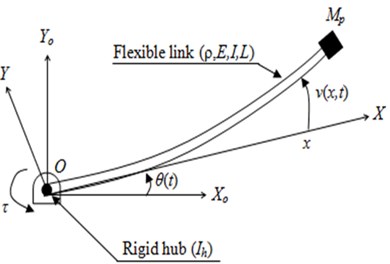
The underwater flexible single-link manipulator system considered in this study is shown in Fig. 1. The link has been modelled as a pinned-free flexible beam. The pinned end of the flexible beam of length $L$ is attached to the hub with inertia $I_h$, where the input torque $\tau \left(t\right)$ is applied at the hub by a motor, and a payload mass $M_p$ is attached at the free end. $E$, $I$ and $\mathrm{\rho }$ represent the young modulus, second moment of inertia and mass density per unit length of the flexible link respectively. $X_0{Y}_0$ axis and $XY$ axis represent the stationary and moving coordinate respectively. Both axes lie in a horizontal plane and all rotation occurs about a vertical axis passing through $o$.

The flexible link, viewed as an Euler-Bernoulli beam, is modeled based on the following assumptions and constraints:

•The flexible link is viewed as a pinned-free flexible beam.

•The flexible link is assumed to be moving in the horizontal plane. So, the perpendicular deformation is neglected.

•Cross-section area and material properties keep constant in each segment.

In order to model the underwater manipulator system efficiently and precisely, it is required to consider an additional forces on the manipulator during motion. These forces, along with the manipulator weight and payload, determine the torques required for generating a motion. There are different forces acting on the manipulator under the water such as lift force, buoyancy and gravity force, fluid acceleration, add mass and drag force [13-15].

Fig. 1Schematic diagram of the flexible single-link manipulator system

Lift force is on the outer way of horizontal plane but perpendicular to the velocity vector. Therefore, the term of the lift force does not appear in the dynamic equations since the movement occurs in the horizontal plane.

Buoyancy is the force which is created due to the volume of the fluid displaced by the submerged body. The buoyant force is acting in opposite direction of the gravity force. Both the gravity and the buoyant forces are not included in the equations because they are opposite to each other and outward direction from the horizontal plane.

Fluid acceleration is produced whenever a fluid is accelerated past a body. The fluid acceleration force is equal to the mass of the water displaced by the body times the acceleration of the fluid and acts in the direction of the fluid acceleration. In the case of a fixed cylinder in an accelerating fluid, there is a fluid-acceleration force (in addition to the added-mass force). For a cylinder accelerating in a still fluid, there is no fluid-acceleration force that accompanies the added-mass force produced. For the research presented here, the fluid was not accelerating, so fluid-acceleration forces were not present.

The mathematical modeling of a land flexible single-link manipulator was derived using a finite element method based on Lagrangian approach [10-12]. The main steps in a finite element analysis can be divided into six sections as follows:

1. Decompose the structure into finite elements, the elements are assumed to be interconnected at certain points, known as nodes. Number of elements determines the accuracy of analyses.

2. For each element, select an approximating polynomials function describing the behavior of the element using an approximation technique to interpolate the result.

3. Formulate the element characteristic matrices and vectors, the equation can be derived from the properties of the material and kinetic and potential energies.

4. Assemble the element matrices and vectors and derivation of system equation, this equation describes the dynamic behavior of the system.

5. Incorporate the boundary condition.

6. Solve the system equation with the inclusion of the boundary condition.

In this manner, the overall approach involves treating the link of the manipulator as an assemblage of $N$ elements of equal length $l=L/N$. For each of these elements the kinetic energy $T_i$ and potential energy $P_i$ are computed in terms of a suitably selected system of five generalized variables $Q$ and their rate of change $\dot{Q}$. The development of the algorithm can be divided into three main steps; finite element method and Lagrangian approach analysis, state space representation and obtaining the result. An outline of this process is given below.

For a small angular displacement $\theta \left(t\right)$ and small elastic deflection $v(x,t)$, the overall displacement $y(x,t)$ of a point along the link at a distance $x$ from the hub can be described as a function of both the rigid body motion $\theta \left(t\right)$ and elastic deflection $v(x,t)$ measured from the line that passing through $o$:

The first step is to find a generalized inertia matrix and a stiffness matrix for a single finite element. As a consequence of using the Euler-Bernoulli beam theory, the finite element method requires each of the nodes through which we divide the beam into elements, to possess two degrees of freedom (DOF), a transverse deflection and rotation. The displacements of the two nodes of the ith element are denoted by $v_n$ and $v_{n+1}$, and the rotations of the nodes by ${\theta }_n$, ${\theta }_{n+1}$. The flexural displacement $v_i(x,t)$ can be described in terms of these DOF and certain shape functions (Hermitian polynomials). In other words, the flexible displacement $v_i(x,t)$ can be approximately expressed as:

where, $s$, represent the local variable, $N_i\left(s\right)$ and $Q_i\left(t\right)$ represent the shape function and nodal displacement respectively. The shape function can be obtained as:

where:

and nodal displacement, $Q_i\left(t\right)={\left[v_n\left(t\right){\theta }_n\left(t\right)v_{n+1}\left(t\right){\theta }_{n+1}\left(t\right)\right]}^T$.

Substituting Eq. (2) into (1) gives:

where:

The new shape function $N_i^{\text{'}}\left(s\right)$ in Eq. (4) and new nodal displacement vector $Q_i^{\text{'}}\left(t\right)$ in Eq. (5) incorporate local and global variables. Among these, the angle $\theta \left(t\right)$ and the distance $x$ are global variables while $N_i\left(s\right)$ and $Q_i\left(t\right)$ are local variables. Define, $s=x-{\sum }_{i=1}^{n-1}{l}_i$ as a local variable of the ith element, where $l_i$ is the length of the ith element. The Eq. (3) and (4) can be expressed as:

According to the basic finite element method and energy principle, the kinetic energy and potential energy of ith element of the link can be acquired according to Eq. (8) and (10) as follow:

where:

is element mass matrix:

where:

is element stiffness matrix and $B_i=d^2{N}_i^{\mathrm{\text{'}}}\left(s\right)/d{s}^2$.

When a body moves relative to the fluid in which it is immersed, a portion of the fluid surrounding the body will moves as well. When a body is accelerated relative to the fluid, the acceleration of the surrounding fluid with the cylinder results in an increase in the force required to produce the acceleration. The added mass effect is normally neglected in land-based robots due to the low density of the air compared to water, while the water can cause much more reaction force for the same manipulator motion. So, added mass has considerable effect in underwater manipulator. The added mass term will be included in the mass term on the left hand side of the equation of motion [16, 17].

Therefore, for the underwater flexible single-link manipulator system, the mass matrix consists of four terms; mass matrix due to the structural mass of the manipulator, mass matrix due to the hydrodynamic added mass, mass matrix due to hub inertia and mass matrix due to tip payload mass. A brief outline of the mass matrices is given below.

The kinetic energy of the ith element due to the structural mass of the manipulator can be obtained using Eq. (8). Thus,

and the element structural mass matrix yields:

where, $A_s$ is the cross section area of the manipulator, and ${\rho }_s$ is the density of the material of the manipulator and:

The kinetic energy of the ith element due to the hydrodynamic add mass can be obtained using Eq. (8). Thus:

and the element add mass matrix yields:

where, $A_f$ is the area that equal to exterior cross section area of the manipulator, ${\rho }_f$ is the density of water, $c_m$ is the hydrodynamic added mass coefficient:

The kinetic energy of tip payload mass can be found using Eq. (16):

where, ${\left[M\right]}_p=M_p{N\text{'}}_i^T{N}_i^{\text{'}}$. Hence, the inertia matrix of tip payload mass $M_p$ is:

Rotational kinetic energy of driving end can be found using Eq. (18):

and the inertia matrix of driving end is expressed as:

Similarly, the potential energy due to the elasticity of the FE can be obtained using Eq. (10) and the element stiffness matrices can be expressed as:

where $E_s$ and $I_s$ are Young Modulus and second moment of inertia of the flexible manipulator respectively.

Summing over all finite elements, the total kinetic and total potential energies $T$ and $P$ of the arbitrary link can be obtained from Eqs. (12), (14), (16), (18) and (20) as:

The global mass matrix has been achieved by assembling the element mass matrices in Eqs. (13) and (15) and modifies it by adding the payload mass matrix Eq. (17) and hub inertia mass matrix Eq. (19) as in Eq. (23):

The global elements stiffness matrix has been achieved by assembling the element stiffness matrix in Eq. (20) as in Eq. (24):

While taking boundary conditions into account, the beam is fixed on one end and there holds ${\theta }_1=v_1=0$. Then ${\theta }_1$ and $v_1$ can be removed from the general coordinates, while the corresponding row and column in the mass matrix and stiffness matrix can also be removed.

The dynamic equations of motion of the flexible manipulator can be derived utilizing the Lagrange equation based on general coordinates:

where $L=T-P$ is the Lagrantian and $F$ is a vector of external forces. Considering the damping, the desired dynamic equations of motion of the system can be obtained as:

where $M^{\mathrm{*}}$ is the global mass matrix, $K^{\mathrm{*}}$ is global rigidity matrix, $D^{\mathrm{*}}$ is structural damping matrix due to structural material, $\left[R\right]$ is the viscous damping matrix due to the fluid drag, $Q^{\mathrm{*}}$ is the general coordinates given as $Q^{*}\left(t\right)=\left[\theta v_2{\theta }_2\cdots \cdots v_N{\theta }_N\right]$ when substituting boundary conditions, $b\mathrm{\text{'}}={\left[\begin{array}{llll}1& 0& \cdots & 0\end{array}\right]}^T$and $\tau$ is input torque.

For the flexible manipulator under consideration, the global mass matrix can be represented as:

where $M_{vv}$ is associated with the elastic degrees of freedom (residual motion), $M_{\theta v}$ represents the coupling between these elastic degrees of freedom and the hub angle $\theta$ and $M_{\theta \theta }$ is associated with the total rotary inertia of the system about the motor axis. Similarly, the global stiffness matrix can be written as:

where $K_{vv}$ is associated with the elastic degrees of freedom (residual motion). It can be shown that the elastic degrees of freedom do not couple with the hub angle through the stiffness matrix. The global damping matrix $D^{\mathrm{*}}$ in Eq. (26) can be represented as:

where $D_{vv}$ denotes the sub-matrix associated with the material damping. The matrix is obtained by assuming that the beam exhibits the characteristics of Rayleigh damping. This proportional damping model has been assumed because it allows experimentally determined damping ratios of individual modes to be used directly in forming the global matrix. It also allows assignment of individual damping ratios to individual modes, such that the total beam damping is the sum of the damping in the modes. Using this assumption, the damping can be obtained as:

where, $\alpha$, and $\beta$, are the Rayleigh damping coefficients related to the modal damping and frequency of the manipulator by:

where ${\zeta }_i$ and ${\omega }_i$ are the ith modal damping ratio and frequency, respectively. Eq. (28) indicates that the more samples of the modal damping ratio and frequency, the more accurate estimation of the Rayleigh damping coefficients. However, it is a common practice in engineering application to use the lower and upper cutoff frequencies of the manipulator system and the corresponding modal damping ratios to define the values of the Rayleigh damping coefficients, such that:

where $\omega$ and $\zeta$ are the modal frequency and damping ratio and the subscripts ‘1’ and ‘2’ are the lower and upper bounds ofthe frequency region in interest, respectively.

There are two types of drag, skin drag which is due to shearing of the fluid in the boundary layer as it flows over the body and pressure drag which is due to the distribution of pressure around the body. For bluff bodies undergoing relatively fast motions, like the cylinders considered here, the flow over the link is separated. Therefore, skin drag is negligible, leaving pressure drag as the primary source of drag. Drag is typically considered as a function of the square of the relative velocity of the body with respect the fluid. The drag torque contribution comes from underwater environment, which is formed because of drag force will be included in the damping term on the left hand side of the equation of motion [16, 18 and 19].

The drag torque is developed on the opposite direction of the links angular velocity. The drag torque matrix of ith element of the link can be acquired according to Eq. (31):

Defining:

Hence:

where:

The $M^{*}$,$\left[D^{*}+R\right]$,$K^{*}$ matrices are of size $m_1\mathrm{*}{m}_1$ and $b\mathrm{\text{'}}={\left[\begin{array}{llll}1& 0& \cdots & 0\end{array}\right]}^T\tau$ has $m_1\mathrm{*}1$ size and $m_1=2n+1$.

Now, the equation of motion is expressed in state-space form, so that it can be solved using control system approaches.

The state-space form of the equation of motion is:

where:

$0_{m1}$ is an $m_1\mathrm{*}{m}_1$ null matrix, $I_{m1}$is an $m_1\mathrm{*}{m}_1$ identity matrix, $I_{2m1}$ is an $2m_1\mathrm{*}2m_1$ identity matrix, $0_{2m1\mathrm{*}1}$ is an $2\mathrm{*}{m}_1\mathrm{*}1$ null vector, and the vector $e$ is the first column of the identity matrix:

3. Simulation results

To study the dynamic behavior of the underwater flexible single-link manipulator system, a computer program was written within Matlab environment and implemented on Intel (R) Core (TM) i7-3612QMCPU @ 2.10GHz processor to simulate the state space matrices derived from the mathematical modeling done above. A cylindrical rod Poly vinyl chloride (PVC) with the specifications shown in Table 1 is considered.

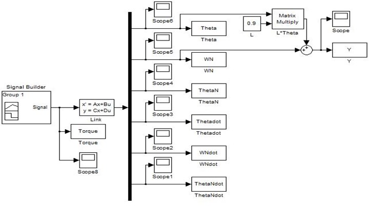
For simplicity purposes, the effects of mass payload and hub inertia are neglected in implementing the simulation algorithm within Matlab as shown in Fig. 2.

Fig. 2SIMULINK diagram of state space matrices

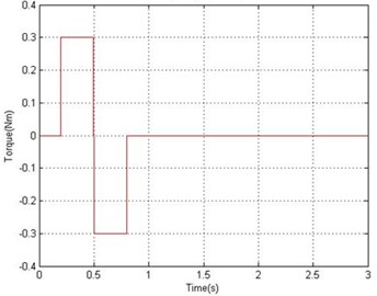
Throughout this simulation, a bang-bang torque input with an amplitude ±0.3 Nm was applied at the hub of the manipulator as shown in Fig. 3. Bang-bang input reflects the nature of the task achieved by the manipulator, i.e. to accelerate from an initial position and then decelerate to a target location. The bang-bang signal is chosen because it consists of one positive pulse and one negative pulse and is considered adequate to study the control performance using this signal. System responses were monitored for the duration of 3 sec with sampling time of 1 msec. To demonstrate the effects of damping on the system response, the responses of the underwater flexible manipulator are observed and recorded for three cases; without the presence of damping, with the presence of structural damping and with the presence of structural damping in addition to drag moment damping in both time and frequency domain respectively.

Fig. 3Bang-bang input torque

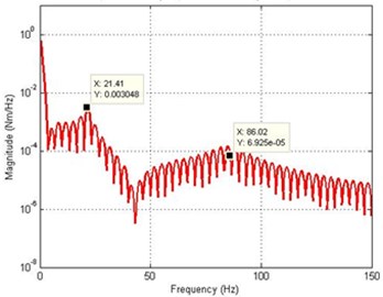
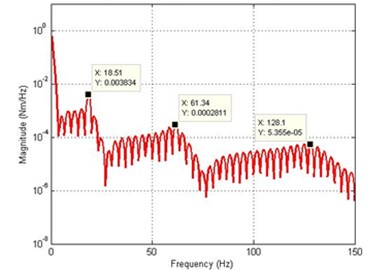
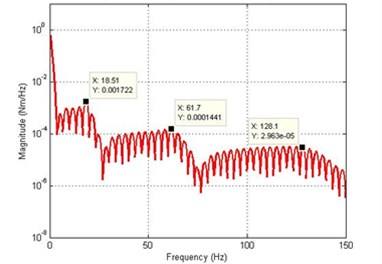
To investigate the accuracy of the FEM simulation in characterizing the behavior of the system, the algorithm was implemented on the basis of varying the number of the element from 1 to 25. Number of elements determines the accuracy of analyses and by increasing the numbers of elements, the system resonance frequencies converge to more accurate values [11]. Resonant frequencies of the system were obtained by transforming the time domain representation of the system into the frequency domain using FFT analysis. The work carried out to show the relation between the resonance modes of the system and the number of element used is summarized in Table 2. It is noted from Table 2 that the number of resonance modes identified increases with an increasing number of elements. A satisfactory dynamic behavior of a flexible manipulator, up to the second mode, could be achieved with one element. Further modes of the system are obtained with increasing the number of elements.The resonance frequency corresponding to the first mode of vibration of the system converges to the reasonably steady value with the algorithm using 2 element or more, for the second mode of vibration with 8 element and for the third mode of vibration 10 element or more.

By increasing the number of elements, the system resonance frequencies converge to more accurate values, but, execution times will be high. This is mainly due to an increase in the size of the mass, damping, stiffness and state-space matrices.

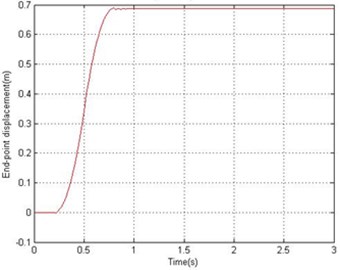
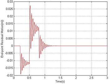
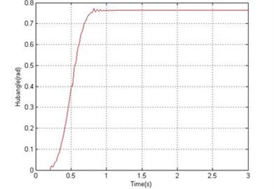
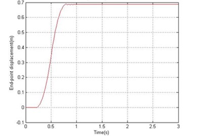
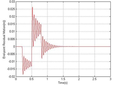
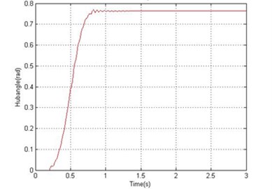
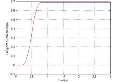
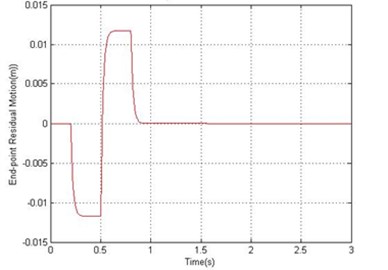
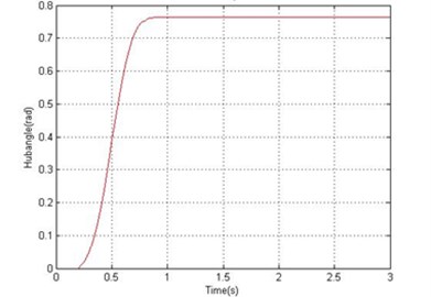
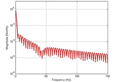
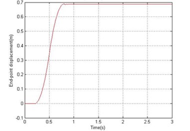
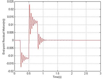
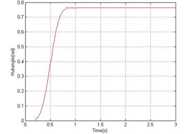
Figs. 4 and 5 show the end point displacement, end point residual motion, hub angle and spectral density of hub angle of the manipulator without the presence of damping using 1 and 10 elements, respectively. It is noted that the response of the system at the end point displacement and hub angle due to the bang-bang torque input reached a steady-state levels of 0.686 m and 0.763 rad respectively, within 0.95 sec using one and ten elements and the system response exhibits persistent oscillation.

Fig. 4Simulated response of the flexible manipulator without damping; Number of elements = 1

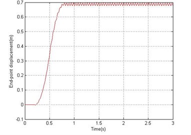
a) End-point displacement

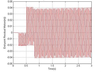
b) End-point residual

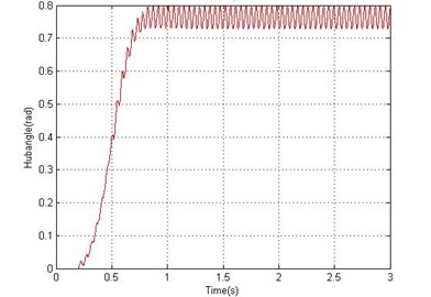
c) Hub angle

d) Spectral density of hub angle

Fig. 5Simulated response of the flexible manipulator without damping; Number of elements = 10

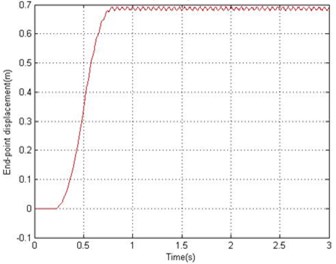
a) End-point displacement

b) End-point residual

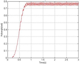
c) Hub angle

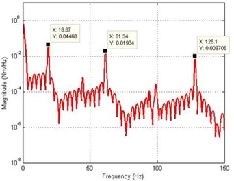
d) Spectral density of hub angle

Fig. 6Simulated response of the flexible manipulator with structural damping; Number of elements =1

a) End-point displacement

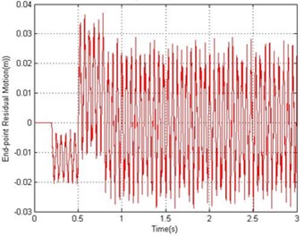
b) End-point residual

c) Hub angle

d) Spectral density of hub angle

Fig. 7Simulated response of the flexible manipulator with structural damping; Number of elements = 10

a) End-point displacement

b) End-point residual

c) Hub angle

d) Spectral density of hub angle

Fig. 8Simulated response of the flexible manipulator with structural and drag torque damping; Number of elements = 1

a) End-point displacement

b) End-point residual

c) Hub angle

d) Spectral density of hub angle

Fig. 9Simulated response of the flexible manipulator with structural and drag torque damping; Number of elements = 10

a) End-point displacement

b) End-point residual

c) Hub angle

d) Spectral density of hub angle

For the dynamic behavior of the system in the presence of structural damping, the damping ratios were assumed as 0.007 and 0.01 for vibration modes 1 and 2 respectively. Using 18.87 Hz and 61.34 Hz as the first two resonance frequencies, $\alpha$ and $\beta$ in Eq. (27) can be obtained as 1.0277 and 4.5170∙${\text{10}}^{\text{-5}}$ respectively. Figs. 6 and 7 show the dynamic behavior of the system in the presence of structural damping with 1 and 10 elements respectively. It is noted from Fig. 7 that the damping has not affected the resonance frequencies of the system, but has resulted in considerable attenuation in the system response amplitude. Analyzing the system time response, it is noted that the hub angle, end point displacement and end point residual motion of the system converged to zero within 1.2 sec.

In fluid dynamics, the drag coefficient (cd) is a dimensionless quantity that is used to quantify the drag or resistance of an object in a fluid environment, such as air or water. In this study, the drag coefficient was assumed as 1.2 to investigate the dynamic behavior of the system in the presence of structural damping and drag torque. Fig. 8 and 9 show the end point displacement, end point residual motion, hub angle and spectral density of hub angle of the manipulator with the presence of structural damping and drag torque using 1 and 10 elements, respectively. It is noted that the damping has reduce the oscillation in the system response. It is also evidenced from the spectral densities of the system response of Fig. 9, that the damping has not affected the resonance frequencies of vibration of the system. However, with damping, the level of vibration reduces as expected.

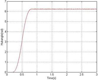
To show the effects of the in-line forces on an underwater flexible single-link manipulator system model, the algorithm was compared with the land flexible single-link manipulator model. A bang-bang torque input with an amplitude ±0.3 Nm was applied at the hub of both underwater and land manipulator as shown in Fig. 3, the responses of the underwater and land flexible manipulator at the hub angle, for five elements, are monitored for duration of 1.3 second with sampling time of 1 msec and recorded as shown in Fig. 10 and Fig. 11 in time domain respectively. It can be noted that the resulted angle for an underwater manipulator was (0.763 rad) and the resulted angle for land manipulator (6.23 rad). That mean, the in-line forces on an underwater single-link manipulator are much larger than the land single-link manipulator. In other word, the torque required for the motion in water is much larger than in air to cope the effect of the in-line forces on an underwater manipulator.

Fig. 10Hub angle response of underwater manipulator

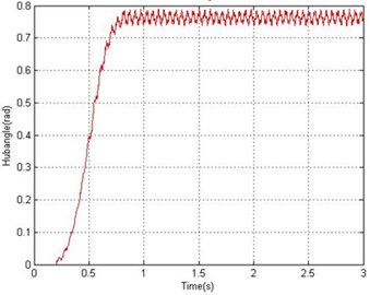
Fig. 11Hub angle response of land manipulator

4. Conclusions

Theoretical investigation into the dynamic characterization of an underwater flexible single-link manipulator system has been presented. A dynamic model of an underwater manipulator has been developed using FEM based on Lagrangian approach. The performance and accuracy of the algorithm have been studied on the basis of varying the number of the element from 1 to 25. It has been demonstrated that by increasing the number of elements, better accuracy in the characterization of the system is achieved but, at the expense of higher execution times. Effects of damping on the system due to structural damping and drag moment damping have been addressed. It is noted that the damping has not affected the resonance frequencies of the system, but has resulted in considerable attenuation in the system response amplitude. Moreover, the effects of the in-line forces on the underwater manipulator were compared with the land flexible manipulator. It has been demonstrated that the in-line forces on the underwater manipulator are much larger than the land manipulator. This study represent the base for further investigations into the application of the modeling approach considered to underwater multilink flexible manipulators and the computational requirements of complex systems of this nature. Moreover, this study can be extended to include the effect of the hub inertia and payload. This simulation platform forms the basis to implement different control structures before online control can be implemented.