Analytical solution for dynamic response of curved rail subjected to moving train

Zhang, Hougui; Liu, Weining; Li, Kefei; Su, Dan

Journal of Vibroengineering

Browse Journal

Submit article

Published: 30 June 2014

Check for updates

Analytical solution for dynamic response of curved rail subjected to moving train

Hougui Zhang¹

Weining Liu²

Kefei Li³

Dan Su⁴

^{1, 2, 3}School of Civil Engineering, Beijing Jiaotong University, Beijing, 100044, China

³Beijing MTR Construction Administration Corporation, Beijing, 100037, China

^{4, 1}Departament of Civil and Environment Engineering, Rutgers, The State University of New Jersey, New Jersey, 08854, USA

Corresponding Author:

Hougui Zhang

Cite the article Download PDF

Downloads 1179

Abstract

The objective of this paper is to present an analytical solution for the dynamic response of curved rail. The detailed solution was derived for the out-of-plane vibration response of periodically supported curved Timoshenko beam subjected to moving loads. The accuracy of the solution was validated based on the results from previous study. Furthermore, the train/track interaction model was introduced into this solution to calculate the rail dynamic response in Beijing metro. The results presented herein indicated that the solution provided accurate results in comparison with both the result from previous study and the measurement data collected from Beijing metro and it can be used to derive the dynamic response for similar situations.

1. Introduction

Rail corrugation, which is found to be very common for curved rails, is becoming an international issue for the railway industry worldwide. In order to investigate the rail corrugation due to the train/track dynamic interaction that was found in Beijing metro, the solution for the dynamic responses of curved rail under moving train loads is needed. In order to focus on the dynamic behavior of track structure, the rail was simplified as a periodically supported Timoshenko beam along horizontally curve, while other external factors, such as the super elevation and the wheel/rail contact condition were not considered in this paper.

Previously, some researchers have been conducted for the out-of-plane vibration of horizontally curved beams. Rao (1971) developed the governing differential equations of motion for the vibration of circular rings based on Hamilton’s principle [1]. Kirkhope (1976), Silva and Urgueira (1988) calculated the nature frequency of out-of-plane curved beams according to Dynamic Reciprocity Theorem [2, 3]. Wang T. M., (1980) also calculated the nature frequency for out-of-plane vibrations of continuous curves beams [4]. Kawakami M. (1995) has investigated both the in-plane and out-of-plane free vibrations of curved beams with variable sections [5]. Yang Y. B. (2001) derived an analytic solution for a horizontal curved simple supported beam subjected to vertical and horizontal moving loads [6]. However, the dynamic response of periodically supported curved Timoshenko beam subjected to moving loads has rarely been studied.

In comparison with the approaches mentioned above, the objective of this paper is to present a solution for the out-of-plane dynamic response of curved rail, which can be simplified as periodically supported curved Timoshenko beam under moving trains load.

In this paper, the general dynamic response of rail induced by moving load along curved path on an elastic semi-infinite space is obtained based on Duhamel Integral and Dynamic Reciprocity Theorem. Regarding periodic track structure, the general dynamic response equation in the frequency domain is simplified in a form of summation within the track sleeper period instead of integral. The transfer function of the curved beam is solved using the transfer matrix approach.

2. Dynamic response of curved beam subjected to moving loads (CBSML)

2.1. Moving load in the semi-infinite space

In the elastic semi-infinite space, as shown in Fig. 1, the vertical load $g (t)$ moves along a curved path with the radius of $R$ , the initial position of $θ_{0}$ , and the angular speed of $c$ . The vertical dynamic displacement of receiver $ξ$ at time-domain can be obtained based on Duhamel integral (Jia Y. X., 2009) [7]:

1

u (ξ, t) = \int_{- \infty}^{+ \infty} g (τ) h_{z} (ξ, θ (τ), t - τ) d τ,

where, $u (ξ, t)$ is the vertical vibration displacement of receiver $ξ$ , and right hand side of Eq. (1) represents the convolution integral of the time history of the moving load $g (t)$ and the vertical transfer function $h_{z} (ξ, θ (τ), t - τ)$ between the time-dependent load position $θ (τ)$ and receiver $ξ$ . Note that, $t - τ < 0$ , $h_{z} (ξ, θ (τ), t - τ) \equiv 0$ .

After transforming the time $t$ to the circular frequency $ω$ , using the Dynamic Reciprocal Theorem and the Forward Fourier Transform, the response displacement in the frequency domain can be expressed as:

2

\hat{u} (ξ, ω) = \int_{- \infty}^{+ \infty} g (τ) {\hat{h}}_{z} (θ_{0} + c τ, ξ, ω) e x p (- i ω τ) d τ,

where, ${\hat{h}}_{z} (θ_{0} + c τ, ξ, ω) = \int_{- \infty}^{+ \infty} h_{z} (θ_{0} + c τ, ξ, t - τ) e x p (- i ω (t - τ)) d t$ is the transfer function in the frequency domain. And the superscript “ $^$ ” is used to indicate the expression in the frequency domain, similarly hereinafter.

Fig. 1Semi-infinite space subjected to moving load

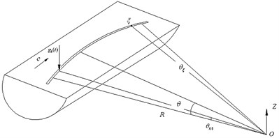
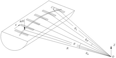
Fig. 2Curved track subjected to moving load

2.2. Moving load on track structure

Since the curved track is symmetric, as shown in Fig. 2, only half of the curved track was considered during analysis. The curved track was subdivided into a number of track cells with the length of $θ_{c e l l}$ , which is the space between sleepers. A vertical load $g (t)$ traversed on the track structure, with the angle speed of $c$ .

According to the relativity of motion, the load moved forward passing over one cell, equivalents to the load itself does not move, while the observation point moves in the opposite direction passing over a cell. Thus, the dynamic response in frequency domain can be simplified in a form of summation with the track sleeper spacing instead of integral, by converting the moving of the load on the rail to the moving of pick-up point by a specific sleeper spacing, which has been proved by the Floquet Transformation (Jia Y. X., 2009) [7].

At time stamp $t$ , the load position in the global coordinate system can be expressed as: $θ = θ_{0} + c t$ , where, $θ_{0}$ is the initial position of the load.

Fig. 3Local coordinate system

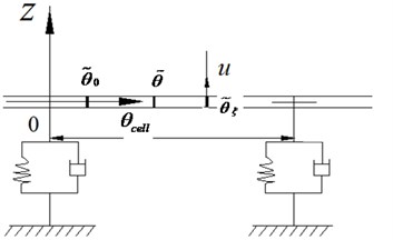
The local coordinate system $\tilde{θ}$ is set up in track basic cell, as shown in Fig. 3. The relationship between the global coordinate system and the local coordinate system can be expressed as follows:

\tilde{θ} = θ - n_{θ} θ_{c e l l}, {\tilde{θ}}_{ξ} = θ_{ξ} - n_{ξ} θ_{c e l l}, {\tilde{θ}}_{0} = θ_{0} - n_{0} θ_{c e l l},

where, “ $~$ ” is used to indicate the expression of the local coordinate system here and throughout this paper, $n_{θ}$ , $n_{ξ}$ , $n_{0}$ are the numbers of basic track cells $θ_{c e l l}$ between the origin and the load position $θ$ , between the origin and the pick-up point $ξ$ , between the origin and the initial load position $θ_{0}$ in the global coordinates, respectively. Thus, the following equation can be developed:

3

t = \frac{θ - θ_{0}}{c} = \tilde{τ} + \frac{(n_{θ} - n_{0}) θ_{c e l l}}{c},

4

\tilde{τ} = \frac{\tilde{θ} - {\tilde{θ}}_{0}}{c} .

According to Eq. (4), when the load moved by one sleeper spacing on the track, the vibration response at receiver $ξ$ can be expressed as:

5

\hat{u} {(ξ, ω)}_{θ_{c e l l}} = \int_{- \infty}^{+ \infty} g (τ) {\hat{h}}_{z} (θ_{0} + c τ, ξ, ω) e x p (- i ω τ) d τ = \int_{0}^{\frac{θ_{c e l l}}{c}} g (\tilde{τ} + \frac{(n_{θ} - n_{0}) θ_{c e l l}}{c}) {\hat{h}}_{z} (θ_{0} + c \tilde{τ} + (n_{θ} - n_{0}) θ_{c e l l}, ξ, ω)

* e x p (- i ω (\tilde{τ} + \frac{(n_{θ} - n_{0}) θ_{c e l l}}{c})) d \tilde{τ} .

In fact, $n_{θ}$ will change when a sleeper spacing was passed over. However, since the curve is not infinitely long and the angle of the curve is $θ_{t}$ , $n_{θ}$ would change from $n_{0}$ to $n_{0} + θ_{t} / θ_{c e l l}$ .

Appling Eq. (4), the expression of the time can be transformed to the expression of space, which can be expressed as:

6

\hat{u} (ξ, ω) = \sum_{n_{θ} = n_{0}}^{n_{0} + θ_{t} / θ_{c e l l}} \frac{1}{c} \int_{{\tilde{θ}}_{0}}^{{\tilde{θ}}_{0} + θ_{c e l l}} g (\frac{(\tilde{θ} - {\tilde{θ}}_{0}) + (n_{θ} - n_{0}) θ_{c e l l}}{c}) {\hat{h}}_{z} (\tilde{θ} + n_{θ} θ_{c e l l}, ξ, ω)

* x p [- i ω (\frac{(\tilde{θ} - {\tilde{θ}}_{0}) + (n_{θ} - n_{0}) θ_{c e l l}}{c})] d \tilde{θ} .

Eq. (6) is the dynamic response of the track structure under vertical moving load in the frequency domain.

2.3. Transfer function of curved track

As proved in previous research (Jia Y. X., 2009) [7], the transfer function ${\hat{h}}_{z} (\tilde{θ}, {\tilde{θ}}_{ξ} + (n_{θ_{ξ}} - n_{θ}) θ_{c e l l}, ω)$ can be solved as the product of the state variables $S (\tilde{θ}, ω)$ at the load excitation point and the transfer function of the periodically supported beam, that can be divided into several basic track cells $θ_{c e l l}$ . Besides that, the transfer function of basic track cell $θ_{c e l l}$ can also be solved as the product of the transfer function of the curved beam and the support under the curved beam, using transfer matrix approach (Sun J. P., 2009) [8] as described below.

2.3.1. The transfer matrix of the curved beam

The curved track is simulated as periodically supported horizontal curved Timoshenko beam. The support under rail is modeled as mass-spring-damper element. For an infinitesimal element of curved beam as shown in Fig. 4, with the length measured along the neutral axis of the curved beam denoted as $s$ , the $x$ -, $y$ - and $z$ - axes are defined as tangential directions, radial and transverse direction, respectively and the origin of the coordinates moves along the neutral axis of the beam. In addition, $u$ is transverse deflection, $α$ is the slope due to pure bending, $φ$ is the angle of torsion, $R$ is the radius and $θ$ is the central angle corresponds to the curve element. It is assumed the cross-section properties and material properties are constant along the beam. The shearing force $Q_{z}$ , bending moment $M_{y}$ and the torsion moment $M_{x}$ are also shown in the Fig. 4.

Fig. 4The coordinates of the curved beam element

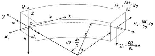
The shear deformation was considered for the analysis of an infinitesimal element $d s$ in the curved beam, $α$ can be expressed:

7

α = v + \frac{\partial u}{\partial x} - \frac{φ x}{R},

where, $ν$ is the transverse shear angle.

And twisting angle $γ$ can be calculated by:

8

γ = \frac{\partial φ}{\partial x} + \frac{1}{R} \frac{\partial u}{\partial x} .

Furthermore, the force-displacement relationship of the curve beam can be obtained from the following equations:

9

Q_{x} = K G A v,

10

M_{y} = - E I_{y} (\frac{\partial α}{\partial x} - \frac{φ}{R}) = E I_{y} (\frac{φ}{R} - \frac{\partial α}{\partial x}),

11

M_{x} = - E I_{s} \frac{\partial^{2} γ}{\partial^{2} x} + G I_{d} (\frac{\partial φ}{\partial x} + \frac{α}{R}),

12

B_{i} = E I_{s} \frac{\partial γ}{\partial x},

where: $E$ is the Young’s modulus, $G$ is the shear modulus; $K$ is the shear correction factor, $I_{y}$ is the vertical bending moment of inertia, $I_{d}$ is free torsion moment of inertia, $I_{s}$ is polar moment of the cross-section and $A$ is the sectional area.

Considering the homogeneous beam with infinite degrees of freedom, the dynamic equilibrium equations of the infinitesimal element of curved beam can be obtained, from its equilibrium condition listed below:

13

\frac{\partial Q_{z}}{\partial x} = ρ A \frac{\partial^{2} u}{\partial t^{2}},

14

\frac{\partial M_{y}}{\partial x} = ρ I_{y} \frac{\partial^{2} α}{\partial t^{2}} + Q_{x} - \frac{M_{x}}{R},

15

\frac{\partial M_{x}}{\partial x} = ρ I_{s} \frac{\partial^{2} φ}{\partial t^{2}} + \frac{M_{y}}{R},

16

\frac{\partial B_{i}}{\partial x} = - M_{x} + G I_{d} γ,

where: $Q_{z}$ is the shearing force, $M_{y}$ is bending moment, $M_{x}$ is torsion moment, $B_{i}$ is double warping moment, $γ$ is warping angle and $ρ$ is the mass per unit volume.

The state vector of any point in the curve beam can be expressed as:

17

S = {Q_{z}, M_{y}, M_{x}, B_{i}, u, α, φ, γ}^{T} .

Thus, Eqs. (7)-(17) can be expressed using matrixes:

18

\frac{\partial S}{\partial x} = A S,

where:

A = [\begin{matrix} 0 & 0 & 0 & 0 & - ρ A ω^{2} & 0 & 0 & 0 \\ 1 & 0 & - \frac{1}{R} & 0 & 0 & - ρ I_{y} ω^{2} & 0 & 0 \\ 0 & \frac{1}{R} & 0 & 0 & 0 & 0 & - ρ I_{s} ω^{2} & 0 \\ 0 & 0 & - 1 & 0 & 0 & 0 & 0 & G I_{d} \\ - \frac{1}{K G A} & 0 & 0 & 0 & 0 & 1 & \frac{x}{R} & 0 \\ 0 & - \frac{1}{E I_{y}} & 0 & 0 & 0 & 0 & \frac{1}{R} & 0 \\ \frac{1}{R K G A} & 0 & 0 & 0 & 0 & - \frac{1}{R} & - \frac{x}{R^{2}} & 1 \\ 0 & 0 & 0 & \frac{1}{E I_{s}} & 0 & 0 & 0 & 0 \end{matrix}] .

The general solution of Eq. (18) can be settled as:

19

S (x) = e^{A x} S_{0},

where, $S_{0}$ is a constant matrix in the solution.

The curved beam can be divided into many infinitesimal elements, with the length of $Δ x$ , and then $x_{k}$ can be expressed as:

20

x_{k} = k Δ x, (k = 1, 2, 3, \dots),

21

x_{k + 1} = x_{k} + Δ x .

Then:

22

S (x_{k + 1}) = T_{i} (Δ x) S (x_{k}),

where, $T_{i} (Δ x) = e^{A Δ x}$ .

Based on the precise integration method of the exponential matrix (Sun J. P. 2009) [8]:

23

T_{i} (Δ x) = e^{A Δ x} = {(e^{\frac{A Δ x}{2^{N}}})}^{2^{N}} = {(e^{A τ})}^{2^{N}},

where, $τ = Δ x / 2^{N}$ , $N =$ 20.

2.3.2. The transfer matrix of the support

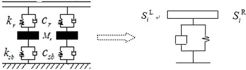
For the periodically supported track structure, the periodic support is simulated as double-layer mass-spring-damper system, in which rail pad and sleeper pad are both modeled as spring-damper element, the sleeper is modeled as concentrate mass between the rail pad and sleeper pad. The double-layer support is calculated as a spring-damper element, as shown in Fig. 5, of which the composite stiffness $k_{v}$ can be expressed as:

24

k_{v} = \frac{c k_{r} \cdot (c k_{s b} - M_{s} ω^{2})}{c k_{r} + (c k_{s b} - M_{s} ω^{2})},

where, $k_{r}$ , $k_{s}$ , $k_{b}$ are the stiffness of rail pad, sleeper pad and subgrade, respectively. $c_{r}$ , $c_{s}$ , $c_{b}$ are the damping of rail pad, sleeper pad, and subgrade , respectively $M_{s}$ is the sleeper mass.

Fig. 5The spring-damper element under the curved beam

Considering an infinitesimal element of the curved beam on the support as shown in Fig. 5, the state vectors of the two sides of the infinitesimal element are defined as follows.

The left side:

25a

S_{i}^{L} = {Q_{i z}^{L}, M_{i y}^{L}, M_{i x}^{L}, B_{i}^{L}, u_{i}^{L}, α_{i}^{L}, φ_{i}^{L}, γ_{i}^{L}}^{T} .

While the right side:

25b

S_{i}^{R} = {Q_{i z}^{R}, M_{i y}^{R}, M_{i x}^{R}, B_{i}^{R}, u_{i}^{R}, α_{i}^{R}, φ_{i}^{R}, γ_{i}^{R}}^{T} .

According to on the continuity requirements:

25c

u_{i}^{R} = u_{i}^{L}, α_{i}^{R} = α_{i}^{L}, φ_{i}^{R} = φ_{i}^{L}, γ_{i}^{R} = γ_{i}^{L}, Q_{i z}^{R} = Q_{i z}^{L} - k_{s l e e p e r} (ω) u_{i},

M_{i y}^{R} = M_{i y}^{L}, M_{i z}^{R} = M_{i z}^{L}, B_{i}^{R} = B_{i}^{L},

where, $k_{s l e e p e r}$ is the composite stiffness of the sleeper that was simplified as spring-damper element. Eq. (25) can be expressed as:

26

S_{i}^{R} = T_{s u p p} S_{i}^{L},

where:

T_{s u p p} = [\begin{matrix} 1 & 0 & 0 & 0 & - k_{s l e e p e r} (ω) & 0 & 0 & 0 \\ 0 & 1 & 0 & 0 & 0 & 0 & 0 & 0 \\ 0 & 0 & 1 & 0 & 0 & 0 & 0 & 0 \\ 0 & 0 & 0 & 1 & 0 & 0 & 0 & 0 \\ 0 & 0 & 0 & 0 & 1 & 0 & 0 & 0 \\ 0 & 0 & 0 & 0 & 0 & 1 & 0 & 0 \\ 0 & 0 & 0 & 0 & 0 & 0 & 1 & 0 \\ 0 & 0 & 0 & 0 & 0 & 0 & 0 & 1 \end{matrix}] .

2.3.3. Initial state vector of the curved beam under unit load

1) Unit load between two sleepers.

As shown in Fig. 6, the state vectors of the double sides of the curve beam element are defined as $S^{L}$ and $S^{R}$ for the left side and for the right side, respectively.

Based on transfer matrix, $S^{R}$ can be calculated as:

27

S^{R} = T_{i} (Δ x) S^{L},

28

S^{R} - S^{L} = P .

Fig. 6Mechanical analysis of the beam element

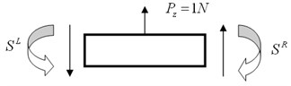
Fig. 7Mechanical analysis of the beam element with support

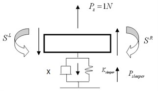
2) Unit load on the sleeper:

29

- Q_{z}^{L} + Q_{z}^{R} + 1 = P_{s l e e p e r} = X k_{s l e e p e r} (ω),

30

S^{R} = T_{i} (Δ x) S^{L},

where, $T_{i} (Δ x) = T_{i} {(Δ x / 2)}^{L} T_{s u p p} T_{i} {(Δ x / 2)}^{R}$ .

Thus the state vector can be settled, as shown in Fig. 7. With the initial state variables and the transfer function of the curved beam settled, the dynamic response of the periodically supported curved track structure under the moving load can be solved.

3. Model validation

Based on the mathematical model described above, the calculation program is developed. In order to validate this model, the rail dynamic responses were calculated and compared with a special case from the literature review. Furthermore, assembled with a well proved vehicle/track interaction model, the rail dynamic response was calculated and compared with the measurement data collected from Beijing metro.

3.1. Model validation based on previous research

Yang Y. B. (2001) [6] proposed an analytical model to calculate the vibration of simple supported curved beam subjected to moving load, as shown in Fig. 8. In order to validate the model in this paper, the example was recalculated with the same input data as below.

Fig. 8Simple supported curved beam

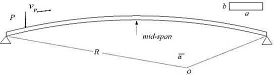
Where, the properties of beam cross section, $a = 5 m,$ $b = 1.8 m,$ $A = a b = 9 m^{2},$ $I_{x} = a b^{3} / 12 = 2.43 m^{4},$ $I_{y} = b a^{3} / 12 = 18.75 m^{4},$ $J_{θ} = I_{x} + I_{y} = 21.18 m^{4},$ the length of beam $L = 24 m,$ the subtended angle $\bar{α} =$ 30° $=$ π/6, the radius $R = 45.84 m,$ Young’s modulus $E = 32.3× 10^{9} N/ m^{2},$ the Poisson ratio $v = 0.2,$ shear modulus $G = E / [2 (1 + v)],$ load $P = 9.8×29.9× 10^{3} N$ , moving speed $V_{p} = 40 m/s$ , and damping $ζ_{d} = 0$ .

As shown in Fig. 9, the mid-span vibration displacement of the simple supported curved beam under moving load is obtained based on the solution developed above.

Fig. 9Displacement response of the simple supported beam

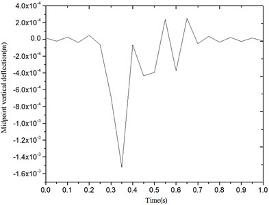
Fig. 10Calculated results by Yang Y. B. (2001)

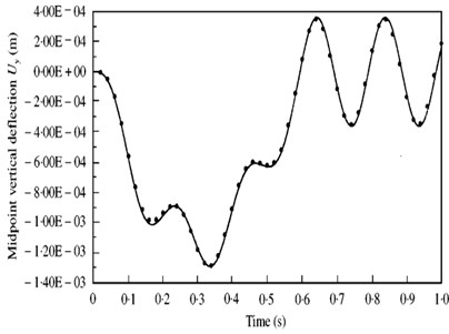
As shown in Fig. 9 and Fig. 10, it is proved that the calculated displacement response has good agreement with the example given by Yang Y. B. (2001) [6], which confirms the reliability of the presented solution.

3.2. Model validation based on measurement data

3.2.1. Assembling the vehicle and CBSML model

In order to further verify the application of the CBSML model, a calibrated vehicle model [9-11] (Fig. 11) was employed into the assembled model to simulate the vertical moving loads on the curved rail. To assemble the vehicle model with CBSML model, Hertz wheel/rail contact model (Fig. 12) is used and the array of the moving load on the rail beam is shown in Fig. 13.

The calculation input data of vehicle model are listed in Table 1, while in the track structure model, $k_{r} =$ 4.2 MN/m, $c_{r} =$ 0.05 MN·s/m, train speed $V =$ 50 km/h, and radii of the curve $R =$ 400 m.

Fig. 11Vehicle model

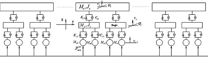
Fig. 12Wheel/Rail Hertz contact model

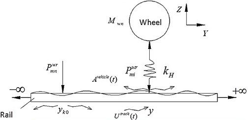
Fig. 13Array of train loads on the rail beam

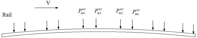
Table 1Parameters of vehicle model

Items	Symbol	Unit	Value
Mass of carriage	$M_{c}$	t	35.0
Carriage mass moment of inertia	$J_{c}$	tm2	1700
Length of carriage	$L$	m	19
Mass of bogie	$M_{t}$	t	4.60
Bogie mass moment of inertia	$J_{t}$	tm2	9.62
Bogie stiffness	$K_{t}$	kN/m	2080
Bogie damping	$C_{t}$	kN∙s/m	240
Space between wheels	$l_{1}$	M	2.20
Space between bogies	$l_{2}$	M	12.6
Wheel mass	$M_{w}$	t	1.42
Wheel stiffness	$K_{w}$	kN/m	2450
Wheel damping	$C_{w}$	kN∙s/m	24

3.2.2. Measurement setup

A campaign of measurement was conducted to estimate the vibration isolation performance of different track forms at the beginning of opening in certain lines in Beijing metro. Therefore, the pass-by rail dynamic responses were collected when both the vehicle and track structure were in good condition. A sharp curve $(R =$ 400 m, $V =$ 50 km/h) was selected as the control measurement section. The fastening systems were directly fixed on the concrete slab without sleeper. The design static stiffness of the fastening system is 4-8 MN/m, but the average static stiffness of 3 systems selected in random from this section is 4.2 MN/mm according to the laboratory test. The detailed measurement condition is listed in Table 2.

Table 2Measurement condition of pass-by rail dynamic response

Item	Value
Radii of curve	400 m
Static stiffness of fastener	4-8 MN/m
Space of fastener	625 mm
Track gauge	1435 mm
Rail	CHN 60 (GB 2585-2007): 60 kg/m
Car marshalling	6 cars (T-M-T-M-M-T)
Axle load	140 kN
Wheel load	70 kN
Bogies space	2.3 m
Train speed at test site	50 km/h

The accelerometer was mounted on the rail with a magnetic support in both vertical and lateral direction, as shown in Fig. 14. However, in this paper, only the vertical rail dynamic response was considered to demonstrate the calculation model.

Fig. 14Accelerometer mounting

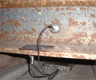
The experimental configuration for the vibration measurements consists of Lance-LC0123T piezoelectric accelerometers and INV3018C dynamic data acquisition system. The accelerometer has the sampling frequency between 0.2 and 11000 Hz, the sensitivity of 26.0 mV/g and the maximum measuring acceleration of 200 g. During the field measurement, the sampling frequency was setup to 5120 Hz, while the sampling distance is 0.625 Hz. The post-processing of the measured data in this paper was carried out in the software DASP, and Hanning window was taken into consideration.

3.2.3. Result comparison

Then the calculated dynamic response results are compared with the measurement data collected from Beijing metro (see Fig. 15) [12].

As shown in Fig. 15, it is observed that there are six wave vibration signals from the calculated time history, each of which corresponds to one car that passed-by. But in raw measurement data, it is hard to clearly distinguish the dynamic response of every car from the irregular signal. It could result from the different of actual axle loads, since the passengers distribute in different cars. However, certain degree of agreement was still observed between raw testing data and analytical results in terms of occurring time and magnitude of the vibration.

Thus, in order to better interpret the testing data and further compare the testing and analytical results, the data was transformed to frequency domain since the frequency spectrum is more interpretable in the analysis of train/track interaction and the estimation of the level of vibration energy. In this study, the frequency spectrum is presented in the form of 1/3 octave band.

Fig. 15Vibration acceleration of curved track under moving train (V= 50 km/h, R= 400 m)

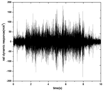
a) Time history (measurements)

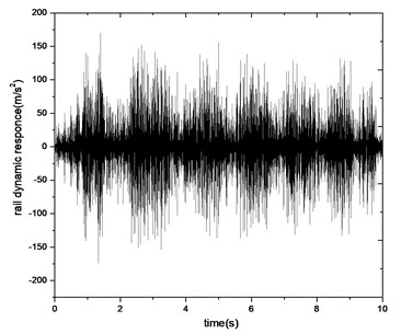
b) Time history (calculation)

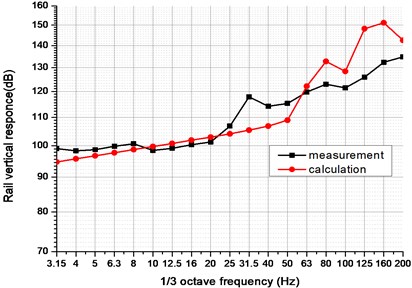
c) Frequency spectrum in 1/3 octave band

From Fig. 15(c), it is clear that the calculated result shows the same tendency with measurement result, especially in the range of 0-25 Hz. As is hardly decayed along the transit path, the low frequency (0-25 Hz) train-induced vibration would cause ground vibration, which generates perceivable vibration and re-radiated noise that would discomfort the occupants in the nearby building. It is indicated that the analytical model could be used to predict the ground vibration problem induced by rail transit systems.

Since the irregularities of track structure and roughness of wheel/rail contact surface were not considered in calculation model, differences were found in the range of 31.5-200 Hz. However, the tendency of both curves is similar and the accuracy of the model would be improved if the roughness of the wheel/rail contact surface is added to the model.

4. Conclusions

An analytical solution was derived for the out-of-plane vibration response of periodically supported curved Timoshenko beam subjected to moving loads. This study is aiming at providing a solution for rail dynamic response of curved rail thereby establish the relationship between the dynamic behaviour and rail corrugation.

The analytical model for vibration of simple supported curved beam under moving load was validated based on results from previous research. Furthermore, in order to further validate the presented solution, a train/track dynamic model was introduced into the assembled model and the calculated results were compared with the measurement data collected from Beijing Metro. The comparison proved that the presented solution could provide accurate results and can be used in future studies.

The advantage of the present approach is that it provides clear mechanism insights into the various vibration phenomena induced by vehicles, in particular, the phenomena of resonance and cancellation, and allows us to identify the key parameters involved.

References

Rao S. S. Eﬀects of transverse shear and rotatory inertia on the coupled twist-bending vibrations of circular rings. Journal of Sound and Vibration, Vol. 16, Issue 4, 1971, p. 551-566.

Search CrossRef
Kirkhope J. Out-of-plane vibration of thick circular ring. Journal of the Engineering Mechanics Division, Vol. 102, Issue EM2, 1976, p. 239-247.

Search CrossRef
Silva J. M. M., Urgueira A. P. V. Out-of-plane dynamic response of curved beams – an analytical model. International Journal of Solids and Structures, Vol. 14, Issue 3, 1988, p. 271-284.

Search CrossRef
Wang T. M., Nettleton R. H., Keita B. Natural frequencies for out-of-plane vibrations of continuous curved beams. Journal of Sound and Vibration, Vol. 68, Issue 3, 1980, p. 427-436.

Search CrossRef
Kawakami M., Sakiyama T., Matsuda H., Morita C. In-plane and out-of-plane free vibrations of curved beams with variable sections. Journal of Sound and Vibration, Vol. 187, Issue 3, 1995, p. 381-401.

Search CrossRef
Yang Y. B., Wu C. M. Dynamic response of a horizontally curved beam subjected to vertical and horizontal moving loads. Journal of Sound and Vibration, Vol. 242, Issue 3, 2001, p. 519-537.

Search CrossRef
Jia Y. X. Study on analytical model of coupled vehicle & track and effect to environment by metro train-induced vibrations. Department of Urban Rail Transit, Beijing Jiao tong University, 2009, (in Chinese).

Search CrossRef
Sun J. P., Li Q. N. Precise transfer matrix method for solving earthquake response of curved Box Bridge. Journal of Earthquake Engineering and Engineering Vibration, Vol. 29, Issue 4, 2009, p. 139-146.

Search CrossRef
Yinxuan Jia, Weining Liu, et al. Influence of vibration on the existing metro structure induced by trains operated on Beijing underground connecting line. China Railway Science, Vol. 29, Issue 5, 2008, p. 72-77, (in Chinese).

Search CrossRef
Yinxuan Jia, Weining Liu, et al. Vibration effect on surroundings induced by passing trains in spatial overlapping tunnels. China Railway Science, Vol. 32, Issue 2, 2009, p. 104-109, (in Chinese).

Search CrossRef
Hougui Zhang Study on effect on nearby metro structures due to train induced vibrations on underground diameter Line in Beijing. The Thesis in Candidacy for the Master Degree of Bridge and Tunneling Engineering, 2007, (in Chinese).

Search CrossRef
Kefei Li, Weining Liu, et al. In-situ test and analysis on the vibration mitigation measures of the elevated line in Beijing metro line 5. China Railway Science, Vol. 30, Issue 4, 2009, p. 25-29, (in Chinese).

Search CrossRef

About this article

Received

11 March 2014

Accepted

20 April 2014

Published

30 June 2014

Keywords

analytical solution

dynamic response

out-of-plane curved beam

moving loads

Acknowledgements

The presented research in this paper was sponsored by National Science Foundation of China (No. 51378001), the Fundamental Research Funds for the Central Universities (No. 20110009120023) and the Fundamental Research Funds for the Central Universities (No. 2013JBM061).

This is an open access article distributed under the Creative Commons Attribution License, which permits unrestricted use, distribution, and reproduction in any medium, provided the original work is properly cited.