Nonlinear dynamics modeling and analysis of disc brake squeal considering acting process of brake force

Liu, Xiandong; Zhao, Yuhan; Shan, Yingchun; He, Tian

Journal of Vibroengineering

Browse Journal

Submit article

Published: 30 June 2014

Check for updates

Nonlinear dynamics modeling and analysis of disc brake squeal considering acting process of brake force

Xiandong Liu¹

Yuhan Zhao²

Yingchun Shan³

Tian He⁴

¹State Key Laboratory of Vehicle NVH and Safety Technology, Chongqing, 400039, China

^{2, 3, 4, 1}School of Transportation Science and Engineering, Beihang University, Beijing, 100191, China

Corresponding Author:

Xiandong Liu

Cite the article Download PDF

Downloads 1130

Abstract

Disc brake squeal of automobile is one of the hottest and most difficult issues concerned by automobile manufacturers and researchers. Considering the acting process of brake force, a simplified nonlinear dynamics model is developed in this paper. The nonlinear dynamics equations are set up and solved by theoretical method and numerical calculation. By studying the effects of key parameters on the system’s behavior, the mechanism of brake squeal are analyzed and discussed. The results indicate that the state of system is more sensitive to the fluctuation of brake force than the variation of the negative slope of friction coefficient against the relative velocity between pad and disc. The dynamic characteristics of brake system are greatly connected with the components stiffness. The brake system may become weakly stable and easily produce brake squeal when tangential contact stiffness, normal contact stiffness and connection stiffness satisfy a certain relationship.

1. Introduction

Brake squeal has become one of the focuses of attention in automotive field for its high frequency characteristic, significant effect on environment and discomfort to people’s feeling. Furthermore, brake squeal decreases the competitiveness of products, which leads many makers of materials for brake pads spending up to 50 % of their engineering budgets on noise issues in brake part design and manufacture [1-2]. Thus, it has been an important research field to develop a new environmental friendly brake system that is quiet but effective.

Unreasonable design of brake, friction materials aging or the change of brake condition may probably cause harsh vibration that may induce brake noise in braking process. The vibration of brake not only includes the friction-induced vibration of materials, but also the part vibration of mechanical components [3]. Automotive brake is a typical dry friction system. In order to investigate the mechanism of noise generation, it is vital to take into account the complex nonlinear characteristics such as friction coefficient against the relative velocity between pad and brake disc [4]. The influence factors are various and many of them are coupled with each other. Thus up to now, there is no widely acceptable mechanism or control methods of brake squeal. But, almost all corresponding papers (even some contradictory literatures) reach a consensus that brake noise has something to do with the friction-induced complex vibration.

The vibration and noise of brake have been widely investigated. There are mainly two methods involved: one is to model the brake system and perform numerical simulation, the other is to carry out bench test and signal analysis. Pertaining to the former, most of the studies focus on linear analyses and searching the stability zone with various parametric conditions to predict the instability. Even though the linear stability theory has been widely applied for analyzing the brake squeal, it may leads to misinterpretation of the dynamics of brake squeal noise [5]. And it is well known that to deeply understand the complicated dynamic characteristics of the brake system a nonlinear model closer to the reality is necessary. Besides, to the best of our knowledge, the generation mechanism about brake squeal and influence rules of key parameters have not been effectually discussed when considering the acting process of brake pressure.

Accordingly, in this paper, the acting process of brake force is introduced, and a nonlinear model of disc brake is established. Then the analytic solution based on the perturbation method is investigated, and numerical simulations are used to verify the analytic solution and to study the effects of some key parameters. Finally, some interesting rules are obtained, and these rules are helpful to understand the mechanism of brake squeal and to design a good quality of disc brake.

2. Simplified dynamic model of brake system

There are several major components of a modern disc brake: the disc (or rotor), caliper, brake pad assemblies and a hydraulic actuation system. The disc is rigidly mounted on the axle hub and therefore rotates with the automobile’s wheel. The pair of brake pad assemblies, which consists of friction material, backing plates and other components, is pressed against the disc in order to generate a frictional torque to slow the disc (and wheel’s) rotation. The caliper houses the hydraulic piston(s) which actuate the pad assemblies. It is attached by a caliper mounting bracket to the vehicle. The methods and points of attachment depend on the type of caliper [6].

Fig. 1 [7] shows a cross-section of a simplified disc brake. The wheel (not shown) is also attached to the rotor, typically at the axle flange. The disc brake shown in this figure has a fixed caliper [7].

Fig. 1Schematic of a simplified disc brake

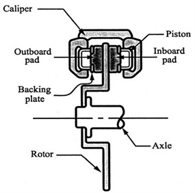
Fig. 2Simplified mechanical model of a disc brake

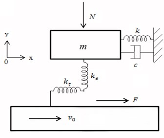
It is acknowledged that brake squeal is mainly related to the brake disc and pad. Thus the disc brake system of automobile may be simplified into a mechanical model such as in Fig. 2.

Assuming that the brake force has not been applied and the spring has no compression, the pad of brake is located at the coordinate system’s origin.

It is conceivable that the friction force is time-varying and depends on some variables. A “good” friction force model is one that captures the essential phenomena and yet not too complicated to render them impractical [8]. The Coulomb friction model, perhaps the simplest friction model, makes distinction between the coefficients of static and kinetic friction. The indeterminate and discontinuous nature of the Coulomb model makes it extremely difficult to simulate the dynamic properties of the mechanical systems when the intermittent stick-slip between two surfaces occurs [9]. Therefore, for dynamic study, the friction model must include velocity dependence at the minimum.

Moreover, in this model, the elastic deformation of the pad or disc is ignored. And what calls for special attention is that the value of normal force on the contact surface between disc and pad is not simply just constant $N$ , but the product of normal contact stiffness and normal displacement written as $k_{e} y$ . Thus, according to Newton’s law, the kinetic equations of the model can be written as:

1

m x + c x + k x + k_{t} x = F (y, v_{r}),

2

m y + k_{e} y = N,

where $v_{r}$ is the difference value between brake disc velocity and tangential velocity of pad: $(v_{0} - x)$ .

$F$ in Eq. (1) is the function of relative velocity $v_{r}$ and normal displacement variables:

3

F (y, v_{r}) = μ ∙ k_{e} ∙ y ∙ s g n (v_{r}) .

Dynamic friction coefficient $μ$ is also the function of relative velocity [10, 11]:

4

μ (v_{r}) = μ_{s} + s g n (v_{r}) ∙ α ∙ v_{r} .

If the negative direction of the relative velocity is considered, the friction force will have a discontinuity at zero relative velocity. This causes the system highly nonlinear and may produce a stick-slip motion.

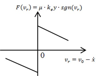
Dynamic friction coefficient $μ (v_{r})$ is shown in Fig. 3. And the friction force $F (v_{r})$ is shown in Fig. 4 without considering the variation of normal force on the contact surface.

Substituting Eq. (3) and (4) into Eq. (1) and (2), the equations become:

5

m \ddot{x} + c \dot{x} + k x + k_{t} x = [μ_{s} + s g n (v_{r}) ∙ α ∙ v_{r}] ∙ k_{e} ∙ y ∙ s g n (v_{r}),

6

m \ddot{y} + k_{e} y = N .

Fig. 3Dynamic friction coefficient μvr

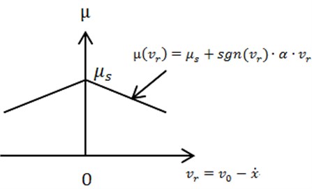
Fig. 4Friction force F(vr)

3. Analytic solution of dynamic model

3.1. Equation solving based on perturbation method

In Eq. (5) there are 2 sign functions which make the nonlinearity stronger. For the convenience of calculation and based on most engineering reality, here we just consider the condition of $v_{0} > \dot{x}$ (i.e. $v_{0} - \dot{x} > 0$ ). Thus $s g n (v_{0} - \dot{x})$ is unity. Considering that the absolute value of friction coefficient’s negative slope is comparatively small, the analytic solution of nonlinear model for brake squeal may be obtained by perturbation method [12].

Rewriting Eqs. (5) and (6) may lead to:

7

m \ddot{x} + c \dot{x} + k x + k_{t} x = [μ_{s} + α ∙ (v_{0} - \dot{x})] ∙ k_{e} ∙ y,

8

m \ddot{y} + k_{e} y = N .

As aforementioned, the value of normal force on the contact surface in Eq. (7) is $k_{e} y$ . While $y$ depends on Eq. (8). So the coupling between Eq. (7) and (8) is established.

In Eq. (8), the initial value of $y$ is zero because the spring has not been compressed until $N$ is applied. Considering the reality and convenience of calculation, $N$ is assumed to be actuated with the step function. With the increase of compression, the force exerted on the contact surface grows synchronously. The response for undamped forced vibration under step excitation can be easily obtained:

9

y = \frac{N}{k_{e}} [1 - \sin (ω_{n} t)],

where, $ω_{n} = \sqrt{k_{e} / m} .$

Substituting Eq. (9) into Eq. (7) which would be rewritten as:

10

\ddot{x} + \frac{c}{m} \dot{x} + \frac{(k + k_{t})}{m} x = \frac{N}{m} [μ_{s} + α ∙ (v_{0} - \dot{x})] [1 - \sin (ω_{n} t)] .

After non-dimensional method is used, we have:

11

\ddot{x} + 2 ζ Ω \dot{x} + Ω^{2} x = G [μ_{s} + α ∙ (v_{0} - \dot{x})] [1 - \sin (ω_{n} t)],

where, $c / m = 2 ζ Ω$ , $(k + k_{t}) / m = Ω^{2}$ , $N / m = G .$

Decomposing Eq. (11) may lead to:

12

\ddot{x} + 2 ζ Ω \dot{x} + Ω^{2} = G (μ_{s} + α v_{0}) [1 - \sin (ω_{n} t)] - G [1 - \sin (ω_{n} t)] ∙ α \dot{x} = [G (μ_{s} + α v_{0}) - G α \dot{x}] + [- G (μ_{s} + α v_{0}) \sin (ω_{n} t) + G \sin (ω_{n} t) α \dot{x}] .

It’s difficult to solve Eq. (12) for its complication. While, each excitation term in the right side of equation is linear except the term $G \sin (ω_{n} t) α \dot{x}$ . Since $α$ is assumed to be very small and the system is weak nonlinear, it may be approximately treated as linear system.

1) Taking the first term on the right side of Eq. (12) as excitation, we have:

\ddot{x} + 2 ζ Ω \dot{x} + Ω^{2} x = G (μ_{s} + α v_{0}) - G α \dot{x} .

Rewriting it leads to:

13

\ddot{x} + (2 ζ Ω + G α) \dot{x} + Ω^{2} x = G (μ_{s} + α v_{0}) .

The solution may be obtained easily:

14

x = \frac{1}{Ω^{2}} [1 - \frac{1}{\sqrt{1 - {(ζ^{'})}^{2}}} e^{- ζ^{'} Ω t} s i n (ω_{d} t + φ)],

where, $ζ^{'} = \frac{2 ζ Ω + G α}{2 Ω}$ , $ω_{d} = Ω \sqrt{1 - {(ζ^{'})}^{2}}$ , $φ = a r c t g \frac{\sqrt{1 - {(ζ^{'})}^{2}}}{ζ^{'}}$ .

2) Taking the second term on the right side of Eq. (12) as excitation, we have:

15

\ddot{x} + 2 ζ Ω \dot{x} + Ω^{2} = - G (μ_{s} + α v_{0}) \sin (ω_{n} t) + G \sin (ω_{n} t) α \dot{x} .

This equation is complex and hard to obtain its solution directly. Since $α$ is assumed to be small enough, that is, this system is weak nonlinear, the perturbation method may be used to get the solution.

Substituting $τ = ω_{n} t$ for the time factor:

\frac{d x}{d t} = ω_{n} \frac{d x}{d τ}, \frac{d^{2} x}{d t^{2}} = {ω_{n}}^{2} \frac{d^{2} x}{d τ^{2}} .

Eq. (15) could be rewritten as:

{ω_{n}}^{2} \ddot{x} + 2 ζ Ω ω_{n} \dot{x} + Ω^{2} x = - G (μ_{s} + α v_{0}) \sin (τ) + G ω_{n} \sin (τ) α \dot{x} .

Setting $Z = Ω / ω_{n}$ and rewriting the equation above, we have:

16

\ddot{x} + 2 ζ Z \dot{x} + Z^{2} x = - \frac{G}{{ω_{n}}^{2}} (μ_{s} + α v_{0}) \sin (τ) + \frac{G}{ω_{n}} α ∙ \sin (τ) \dot{x} .

Eq. (16) can be simplified as follow:

17

\ddot{x} + 2 ζ Z \dot{x} + Z^{2} x = A \sin (τ) + ε ∙ \sin (τ) \dot{x},

where, $A = - \frac{G}{{ω_{n}}^{2}} (μ_{s} + α v_{0})$ , $ε = \frac{G}{ω_{n}} α .$

$ε$ can be treated as perturbation factor for the small $α$ . The solution of equation $x (τ)$ becomes:

18

x (τ) = x_{0} (τ) + ε x_{1} (τ) + ε^{2} x_{2} (τ) + ε^{3} x_{3} (τ) + \dots .

Substituting Eq. (18) into both sides of Eq. (17), we get the left side terms:

({\ddot{x}}_{0} + 2 ζ Z {\dot{x}}_{0} + Z^{2} x_{0}) + ε ({\ddot{x}}_{1} + 2 ζ Z {\dot{x}}_{1} + Z^{2} x_{1}) + ε^{2} ({\ddot{x}}_{2} + 2 ζ Z {\dot{x}}_{2} + Z^{2} x_{2}) + \dots,

the right side terms:

A \sin (τ) + [ε \dot{x_{0}} (τ) + ε^{2} \dot{x_{1}} (τ) + ε^{3} \dot{x_{2}} (τ) + \dots] \sin (τ) .

Recognizing that the resulting equation must be satisfied for all values of $ε$ and that the functions $x_{i}$ ( $i =$ 0, 1, 2, …) are independent of $ε$ , it follows that the coefficients like powers of $ε$ on both sides must be equal to one another. Thus the equation becomes a set of equations:

{\ddot{x}}_{0} + 2 ζ Z {\dot{x}}_{0} + Z^{2} x_{0} = A \sin (τ),

{\ddot{x}}_{1} + 2 ζ Z {\dot{x}}_{1} + Z^{2} x_{1} = {\dot{x}}_{0} (τ) \sin (τ),

{\ddot{x}}_{2} + 2 ζ Z {\dot{x}}_{2} + Z^{2} x_{2} = {\dot{x}}_{1} (τ) \sin (τ) .

The equations above are all oscillation equations of damped system under periodic excitation. And their solutions can be easily got respectively:

x_{0} (τ), x_{1} (τ), x_{2} (τ), x_{3} (τ) \dots .

Substitution of these solutions into Eq. (18) leads to the response of system:

19

x (τ) = A_{0} A s i n (τ - φ_{0}) + ε \frac{A_{0} A}{2} [A_{1} \sin (2 τ - φ_{1}) + \frac{1}{Z^{2}} \sin (φ_{0})]

+ ε^{2} \frac{A_{0} A_{1} A}{2} [A_{2} \sin (3 τ - φ_{2}) - A_{0} \sin (τ - φ_{1} - φ_{0})] + \dots,

where:

A_{0} = \frac{1}{\sqrt{{(Z^{2} - 1)}^{2} + {(2 ζ Z)}^{2}}}, φ_{0} = a r c t g (\frac{2 ζ Z}{Z^{2} - 1}),

A_{1} = \frac{1}{\sqrt{{(Z^{2} - 4)}^{2} + {(4 ζ Z)}^{2}}}, φ_{1} = a r c t g (\frac{4 ζ Z}{Z^{2} - 4}) + φ_{0},

A_{2} = \frac{1}{\sqrt{{(Z^{2} - 9)}^{2} + {(6 ζ Z)}^{2}}}, φ_{2} = a r c t g (\frac{6 ζ Z}{Z^{2} - 9}) + φ_{0} + φ_{1} .

3.2. Analysis of system’s solution

1) Eq. (14) is one part of system’s solution. We may conclude from the expression that exponent term $e^{- ζ^{'} Ω t}$ has a significant influence on the response characteristics. Considering the value of exponent power, we have:

- ζ^{'} Ω = - \frac{2 ζ Ω + G α}{2 Ω} Ω .

As aforementioned: $c / m = 2 ζ Ω$ , $N / m = G$ , the expression may be rewritten as:

- ζ^{'} Ω = - \frac{c + N α}{2 m} .

If $c + N α < 0,$ i.e. $c < - N α = N |α|,$ $- ζ^{'} Ω > 0,$ so the system is divergent; and if $c + N α > 0$ , i.e. $c > - N α = N |α|$ , $- ζ^{'} Ω < 0$ , so system is convergent.

Thus the following conclusions may be reached: in general, the stability of system depends on the value of damping, brake force and the negative slope of friction coefficient. If the product of brake force $N$ and slope $|α|$ is greater than the damping coefficient $c$ , the system’s response may become divergent and the vibration is intensified.

Obviously, the relation and values of brake force $N$ , slope $|α|$ and damping coefficient $c$ are very vital to the propensity of brake squeal.

2) Eq. (19) is the other part of system’s solution.

As aforementioned equation:

Z ＝ \frac{Ω}{ω_{n}},

we have:

Z^{2} = \frac{Ω^{2}}{{ω_{n}}^{2}} = \frac{(k + k_{t}) / m}{k_{e} / m} = \frac{k_{t} + k}{k_{e}} .

Setting:

β = \frac{k_{t}}{k_{e}}, γ = \frac{k}{k_{e}},

then the following is induced:

Z^{2} = β + γ .

Obviously, if $Z^{2} = β + γ = n^{2}$ , ( $n =$ 1, 2, 3, …), $A_{0}$ , $A_{1}$ , $A_{2}$ ,… in Eq. (19) will become infinite, which means $x (τ)$ is at its maximum. Under this situation the system will be instable and easily induce brake squeal.

Accordingly, the dynamic characteristics of disc brake system are greatly connected with the components stiffness. Increasing only the stiffness of one part may cause a significant squeal noise. The relations of corresponding stiffness variables should be deliberately designed: if the sum of $β$ (the ratio of tangential contact stiffness to normal contact stiffness between brake disc and pad) and $γ$ (the ratio of connection stiffness between pad and caliper brake anchor to normal contact stiffness between brake disc and pad) satisfies some certain relations, the brake system may become unstable and produce brake squeal.

4. Numerical simulations of dynamic model

To further investigate the effects of model’s parameters on brake squeal and verify the conclusion of previous analyses, the numerical simulations are performed. Introducing the friction model, the nonlinear differential Eqs. (5) and (6) may be rewritten in the form of state equations as follows:

20

\dot{x_{1}} = x_{2},

\dot{x_{2}} = - \frac{c}{m} x_{2} - \frac{β + γ}{m} k_{e} x_{1} + \frac{[μ_{s} + s g n (v_{0} - \dot{x}) ∙ α ∙ (v_{0} - \dot{x})] ∙ k_{e} y ∙ s g n (v_{0} - \dot{x})}{m},

\dot{x_{3}} = x_{4},

\dot{x_{4}} = - {\frac{k_{e}}{m} x}_{3} + \frac{N}{m} .

As previously mentioned, the condition of $v_{0} > \dot{x}$ (i.e. $v_{0} - \dot{x} > 0$ ) is introduced in the analytic solutions. But here, for the convenience of simulation and requirement of precise results, the value of $\dot{x}$ is not limited. Thus, the sign function will be taken into account.

Besides, the self-excited vibration does not always produce the stick-slip instability, but also produce the steady limit cycle. Linear analysis may show the system is unstable while the size of limit cycle is very small and may produce inaudible sound. Thus, it is believed that the size of limit cycle is more important than the existence of limit cycle [5]. Accordingly, in this paper, the size of limit cycle is also considered to describe more understandable mechanisms of squeal noise. It shows that: the system tends to be instable easier when its size of limit cycle is bigger. Thus, numerical simulation is carried out to demonstrate the effects of some key factors, such as negative friction coefficient $α$ , brake force $N$ and contact stiffness $k_{e}$ .

Note that in these numerical examples, the stiffness is deliberately taken to be very small without losing the generality. And this will not affect the qualitative features of the results or conclusion drawn from the results thus obtained [5, 13]. Besides, the precise relationship of stiffness is ignored and all the stiffness values are set equal in the following numerical study. Further discussion about stiffness will be performed later. The value table is shown as Table 1.

Table 1Basic parameters for numerical simulation

$m$ (kg)	$c$ ( $N∙s∙ m^{-1}$ )	$v_{0}$ ( $m∙ s^{-1}$ )	$μ_{s}$	$k_{e}$ ( $N∙ m^{-1}$ )	$k_{t}$ ( $N∙ m^{-1}$ )	$k$ ( $N∙ m^{-1}$ )	$β$	$γ$
0.3	0.01	1	0.3	1	1	1	1	1

4.1. The effects of $N$ and $α$ on system’s dynamic characteristics and sensitivity analysis

Previous analyses draw a conclusion that increasing $N |α|$ may cause the negative influences to system’s stability. And $|α|$ is assumed comparatively small. Here, we will study vibration solutions at different values of $|α|$ and $N$ , proceeding by varying one parameter while keeping the other constant. In order to compare the sensitivity of system response introduced by them respectively, their values are set to increase at the same rate.

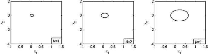
1) $α$ is fixed as –0.002, and the values of $N$ is various: $N =$ 1, 2, 5, 10, 20, 50 N.

System’s phase diagrams are plotted as Fig. 5 by displacement $x_{1}$ on the horizontal axis and velocity $x_{2}$ on the vertical.

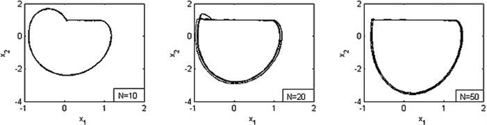
From these figures, it can be seen that the limit cycle occurs when $N$ is less than 5 (i.e. $N |α| < c = 0.01$ ). And as increasing the value of brake force $N$ , the size of limit cycle increases apparently, either. It means the displacement and velocity increase gradually. If $N$ is more than 5 (i.e. $N |α| > c = 0.01$ ), the stick-slip motion occurs and the amplitude of vibration increases with $N$ .

Fig. 5Phase diagrams for various values of N, where α= –0.002

a)

b)

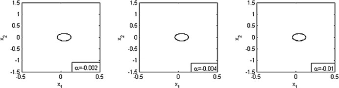
2) $N$ is fixed as 1 N, and the values of $α$ is various: $α =$ –0.002, –0.004, –0.01, –0.02, –0.04, –0.1. System’s phase diagrams are plotted as Fig. 6.

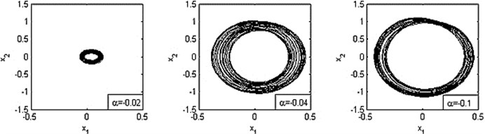
These figures show that the limit cycle occurs when $|α|$ is less than 0.01 (i.e. $N |α| < c = 0.01$ ). And the size of limit cycle increases with $|α|$ ’s growth. If $|α|$ is more than 0.01 (i.e. $N |α| > c = 0.01$ ), the amplitude of vibration becomes greater during $|α|$ ’s growth and the motions are complex (quasi-periodic motion or chaotic motion).

Based on above analyses, the following conclusions may be obtained:

1) Limit cycle occurs and remains when $N |α|$ is less than a critical value and the role of $N$ is more subtle. Numerical results show that the size of limit cycle grows with the increase of $N$ , while there is no evident change of the cycle’s size during $|α|$ ’s increase in the meantime. Moreover, by keeping $N |α|$ constant, the amplitude of vibration is found to be larger at greater $N$ compared with greater $|α|$ . And it indicates that the system may become unstable and brake squeal is more easily to be induced under $N$ ’s severe variation.

2) As to the characteristics of system’s phase diagrams, when $N$ is various and $|α|$ is fixed, stick-slip is much more obvious if the product of $N$ and $|α|$ is over the critical value. When keeping $N$ constant, there is a tendency to be complex motion (quasi-periodic motion or chaotic motion) if $N |α|$ exceeds the threshold.

Fig. 6Phase diagrams for various values of α, where N=1

a)

b)

One thing to note here is that: without considering the sign function, there may be some deviation between the result of analytic solution and numerical simulation. While, in this paper, the threshold value of $N |α|$ happens to be $c$ for the particular selection of parameters. And the threshold may be different if the values of parameters change. But the tendency of motion won’t be greatly affected and the identification of critical value needs further investigation.

Generally, the state of system is more sensitive to the fluctuation of brake force than the variation of the negative slope of friction coefficient against the relative velocity. Thus it can be seen that the fluctuation of $N$ may decrease the stability of system during the braking, and could be a more significant factor inducing brake squeal compared with $α$ .

Fig. 7Phase diagrams for various values of stiffness

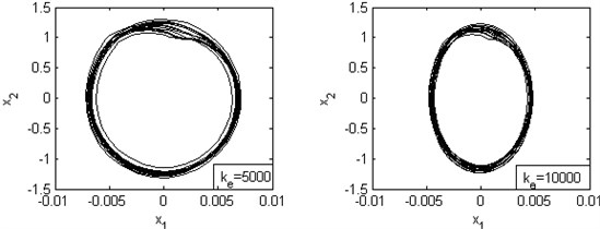
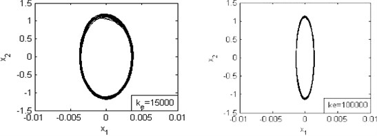
4.2. The effects of stiffness on system’s dynamic characteristics

The connection stiffness $k$ between pad and caliper brake anchor, the tangential contact stiffness $k_{t}$ and normal contact stiffness $k_{e}$ between brake disc and pad are assumed to be identical. The ratios are set to $β = k_{t} / k_{e} = 1$ , $γ = k / k_{e} = 1$ .

Based on this assumption, the other parameters are set to $α =$ –0.15, $N =$ 100. For the cases of $k_{e} =$ 5000, 10000, 15000, 100000, the simulation results are shown in Fig. 7.

Fig. 7 shows a complex state of system’s motion. And the limit cycle becomes apparent as the increasing of the stiffness value. So, we may guess that the enhancement of stiffness may weaken the complex motion and decrease the displacement. And it’s helpful to prevent the system from unstable state and minimize the occurrence of the squeal noise.

4.3. The effects of $β$ and $γ$ on system’s dynamic characteristics

In section 3.2, the conclusion is obtained that the condition of $Z^{2} = β + γ = n^{2}$ ( $n = 1, 2, 3,…$ ) will induce stronger vibration. To make clear how the parameters $β$ and $γ$ influence the system’s dynamic characteristics, the phase diagrams of system are simulated for various $β$ and $γ$ .

In section 4.1 and 4.2, $β$ and $γ$ are set to be equal. However, for the real brake system, the tangential contact stiffness between brake disc and pad will be no more than the normal one, namely $β <$ 1 (usually between 0.25 and 0.64) [14].

So, considering the real range of stiffness value, the situations when $n =$ 2, 3, … are ignored. Here we just study the condition when the sum of $β$ and $γ$ is around 1. And the parameters like $k_{e}$ , $N$ and $α$ are fixed to be constant ( $k_{e} =$ 1, $N =$ 1, $α =$ –0.002).

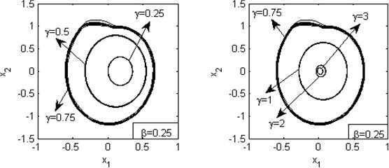
First, the ratio $β$ of tangential contact stiffness to normal contact stiffness between brake disc and pad is fixed to be constant 0.25. And $γ$ is set to be 0.25, 0.5, 0.75, 1, 2, 3 respectively. Fig. 8 shows the results.

Fig. 8Phase diagrams for various values of γ, where β=0.25

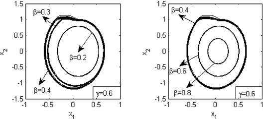
Then, the ratio $γ$ of stiffness between pad and caliper brake anchor to normal contact stiffness between brake disc and pad is fixed as constant 0.6. And $β$ is set to be 0.2, 0.3, 0.4, 0.6, 0.8 respectively. Fig. 9 shows the results.

From these figures, a very important phenomenon can be found: $β + γ = 1$ becomes a boundary point of making the vibration larger and more unstable. Since the size of limit cycle is related to the amplitude of instability, increasing $β$ or $γ$ may stabilize the unstable vibrations for the case of $β + γ > 1$ . On the contrary, it could weaken the stability if $β + γ <$ 1.

Specifically, if the contact stiffness is fixed and the connection stiffness $k$ is small enough to lead to $β + γ < 1$ , improving the value of $k$ may make the vibration much more severe. However, if the connection stiffness $k$ is fixed great, reasonably choosing the materials of pad and disc of higher $β$ may enhance system’s stability and reduce the occurrence of brake squeal.

Briefly speaking, it is emphasized that the relationship between contact and connection stiffness must be carefully considered. And it’s beneficial to minimize the possibility of brake squeal if the sum of $β$ and $γ$ is away from 1. Obviously, the simulation’s result corresponds to the conclusion of analytic solution about the effect of $β$ and $γ$ on the system’s stability.

Fig. 9Phase diagrams for various values of β, where γ=0.6

4.4. Bifurcation numerical simulation

Bifurcation is usually seen as the point in which the number of fixed point and/or (quasi-) periodic solutions changes. It has a close relation with the generation of self-excited vibration in engineering [15].

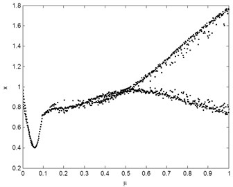
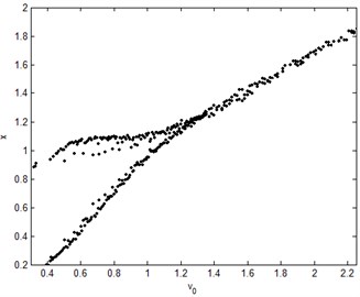
When $α =$ –0.02, $k_{e} =$ 1, $β + γ = 1$ , the bifurcation diagram can be studied with the dynamic friction coefficient and the driving speed of the disc as bifurcation parameters. The results are shown in Figs. 10(a)-(b).

Fig. 10(a) shows that the system approximately appears the period-doubling bifurcation when the dynamic friction coefficient reaches 0.32. The bifurcation diagram can be divided into two areas of 0 $< μ <$ 0.32 and 0.32 $< μ <$ 1 with different characteristics. The results show that the system tends to stable when $μ$ is less than the critical value.

Likewise, Fig. 10(b) shows that the approximately period-doubling bifurcation has occurred in the region of 0 $< v_{0} <$ 1.38. The system will be stable when the driving speed of disc is more than the certain value.

Fig. 10Bifurcaion diagrams with: a) dynamic friction coefficient and b) driving speed of disc as the bifurcation parameter

a)

b)

5. Conclusions

Considering the step brake force, a simplified nonlinear dynamics model is developed. The dynamics equations are set up and solved with theoretical solution and numerical calculation. By studying the effects of key parameters on the system’s behaviors, the mechanism of brake squeal is analyzed and discussed.

The result indicates that:

1) The system is relatively stable if the product of brake force $N$ and $|α|$ is less than a threshold. If it exceeds this critical value, the vibration becomes worse and easily induces brake squeal.

2) Compared to the variation of $|α|$ at the same condition, the state of system is more sensitive to the fluctuation of brake force.

3) The dynamic characteristics of system have something significant to do with tangential and normal contact stiffness between brake disc and pad, and connection stiffness between pad and caliper brake anchor. Increasing only one component’s stiffness may not necessarily avoid the brake squeal. And the relationship between contact and connection stiffness must be deliberately considered. If the sum of $β$ and $γ$ is close to 1, the vibration may become unstable and brake squeal is likely to occur.

4) The system tends to be stable when the dynamic friction coefficient is less than a critical value or the driving speed of disc is more than a certain value.

Although the motivation for our work is based on studies of a simple model for a brake system, we are pursuing a more specific relationship between the response and key parameters. In this paper, the tangential contact stiffness between the disc and pad is taken into consideration and is deeply researched, but these are seldom performed in other literatures. Based above investigations, the equation of stiffness relation $β + γ = 1$ is proposed as the unstable criterion. Besides, the sensitivity analysis of $N$ and $|α|$ gives an inspiration for the further study. The fluctuation of brake force should be paid more attention in the brake squeal analysis.

References

Abendroth H., Wernitz B. The integrated test concept: dynovehicle, performance-noise. SAE Paper, 2000, p. 2000-01-2774.

Search CrossRef
Fenghong Y., Wei Z. Nonlinear dynamical analysis for a disc braking system. Journal of Vibration and Shock, Vol. 28, Issue 6, 2009, p. 93-94, 99, (in Chinese).

Search CrossRef
Tao W., Wenjian Z. Friction brake-theory, structure and design. South China University of Technology Press, Guang Zhou, 1992, (in Chinese).

Search CrossRef
Xiaobin N., Wenming Z. Muti-body dynamic simulation for analysis of disc brake vibration. Nonferrous Metals, Vol. 56, Issue 4, 2004, p. 119-121, (in Chinese).

Search CrossRef
Kihong S., Jae-Eung O. H., Michael J. B. Nonlinear analysis of friction induced vibrations of a two-degree-of-freedom model for disc brake squeal noise. JSME International Journal, Vol. 45, Issue 2, 2002, p. 426-432.

Search CrossRef
Kinkaid N. M., O’Reilly O. M., Papadopoulos P. Automotive disc brake squeal. Journal of Sound and Vibration, Vol. 267, 2003, p. 105-166.

Search CrossRef
Kinkaid N. M. On the nonlinear dynamics of disc brake squeal. University of California, Berkeley, 2004.

Search CrossRef
Li Y., Feng Z. C. Bifurcation and chaos in friction-induced vibration. Communications in Nonlinear Science and Numerical Simulation, Vol. 9, Issue 6, 2004, p. 633-647.

Search CrossRef
Shaw S. W. On the dynamic response of a system with dry friction. Journal of Sound and Vibration, Vol. 108, 1986, p. 305-325.

Search CrossRef
Thee S. K., Tsang P. H. S., Wang Y. S. Friction induced noise and vibration of disc brakes. Wear, Vol. 133, 1989, p. 39-45.

Search CrossRef
Ouyang H., Cartmell M. P., Friswell M. I., Mottershead J. E. Friction-induced parametric resonances in discs: effect of a negative friction-velocity relationship. Journal of Sound and Vibration, Vol. 209, Issue 2, 1998, p. 251-264.

Search CrossRef
Meirovitch L. Fundamentals of vibration. McGraw Hill, 2001.

Search CrossRef
Ouyang H., Mottershead J. E., Cartmell M. P., Brookfield D. J. Friction-induced vibration of an elastic slider on a vibrating disc. International Journal of Mechanical Sciences, Vol. 41, Issue 3, 1999, p. 325-336.

Search CrossRef
Rusli M., Okuma M. Squeal noise analysis in mechanical structure with friction: prediction by experiment-based method of structural analysis. Saarbrücken, VDM Verlag Dr. Müller, 2010.

Search CrossRef
Xiaopeng L., Guanghui Z., Xing J., Yamin L., Hao G. Dynamics of mass-spring-belt friction self-excited vibration system. Journal of Vibroengineering, Vol. 15, Issue 4, 2013, p. 1778-1789.

Search CrossRef

About this article

Received

06 January 2014

Accepted

13 April 2014

Published

30 June 2014

Keywords

brake squeal

nonlinear

disc brake

modelling

Acknowledgements

The authors would like to thank the financial support provided by the opening project of Beijing Higher Education Young Elite Teacher Project (Grant No. YETP1116), State Key Laboratory of Vehicle NVH and Safety Technology of China (No. NVHSKL-201108) and the Natural Science Foundation of China (No. 51275022).

This is an open access article distributed under the Creative Commons Attribution License, which permits unrestricted use, distribution, and reproduction in any medium, provided the original work is properly cited.