Abstract
This paper presents a dynamical model for an especially designed motorized spindle with an adjustable preload mechanism and analyzes the effects of bearing preload on the spindle dynamical properties in both of the non-working and working states. In the model, the housing, rear bearing pedestal, shaft, drawbar and tool are taken into account using the finite element (FE) method. The effects of bearing preload are provided by this mathematical model as well as the experiments, in which the axial displacement of spindle tool, frequency response function (FRF), vibration displacement etc. are measured under all kinds of operating conditions. Various results such as bearing nonlinear stiffness, inherent modal shapes and frequencies of the system, spindle stiffness and chatter stability have been obtained under different preload. The good agreement between the calculated results and the tested data indicates that the model is capable of predicting the dynamical properties of the motorized spindle system accurately. And it is indicated that choosing an appropriate bearing preload can contribute to acquire good dynamical properties for the motorized spindle.
1. Introduction
High speed machining (HSM) is widely used in the aeronautical and automotive domains to increase productivity and reduce production costs, in which the motorized spindle system is one of the most important parts since its dynamical properties directly affect the machining productivity and finish quality of the workpieces [1]. And the preload of angular contact ball bearing, usually used in the motorized spindle, has a great influence on the dynamical properties of system. Therefore, there is a necessity of comprehensive and in-depth study on the dynamical properties analysis of motorized spindle under different bearing preload.
In early spindle dynamical analysis, bearings are usually assumed that under invariable preload and simplified into springs with constant stiffness, and shafts are regarded as ideal or simple shapes [2-3]. With the in-depth study on rolling bearings, the centrifugal force and gyroscopic moment of the rolling element caused by the high speed are taken into account. Jones A. [4] established the quasi static model of radial rolling bearings and analyzed the load distribution of the rolling elements. And using this model, Li S. S. et al. [5] calculated the stiffness of the bearings at very high speed and found that the preload of bearing have significant influence on bearing stiffness. With the in-depth study on dynamics of rotor, shear effect and gyroscopic effect have been considered, and those rotors was called Timoshenko beam [6]. Using the quasi static model of bearing and Timoshenko beam theory, more and more scholars took the effect of thermal effects into account to study the dynamical properties of motorized spindle [7-9]. Chen X. A. et al. [10] proposed an integrated model which consists of four coupled sub-models: state, shaft, bearing, and thermal model, and analyzed the effects of thermal expansion, unbalanced magnetic force and high speed on the bearing preload state and dynamical properties of the motorized spindle system. For analyzing the effects of different preload mechanisms on the dynamical properties of motorized spindle, Cao H. R. et al. [11] established the mathematic models for both of the bearing “constant” and “rigid” preload mechanisms and found that at high speed and under cutting loads the “rigid” preload mechanism has more efficient dynamic stiffness of spindles than “constant” preload. Chen J. S. and Chen K. W. [12] designed a bearing preload monitoring and control mechanism, using an integrated strain-gage load cells and piezoelectric actuators, to seek the perfect preload and obtained good machining quality.
All of the researches mentioned above predict inherent characteristics for a spindle system, and consider only the shaft and bearings. The effects of the housing, tool and drawbar on the spindle dynamics are neglected. Meanwhile, the “constant” and “rigid” preload mechanisms could not represent all the preload state of bearing, and an adjustable preload mechanism is needed. Therefore, this paper, aiming at the problems mentioned above, presents a dynamical model for an especially designed motorized spindle with an adjustable preload mechanism and analyzes the effects of bearing preload on the spindle dynamical properties in both of the non-working and working states. Various results such as bearing nonlinear stiffness, inherent modal shapes and frequencies of the system, spindle stiffness and chatter stability have been obtained under different preload and all kinds of operating conditions. From the calculated and tested data, it can be indicated that choosing an appropriate bearing preload can contribute to acquire good dynamical properties for the system.
2. Dynamical model
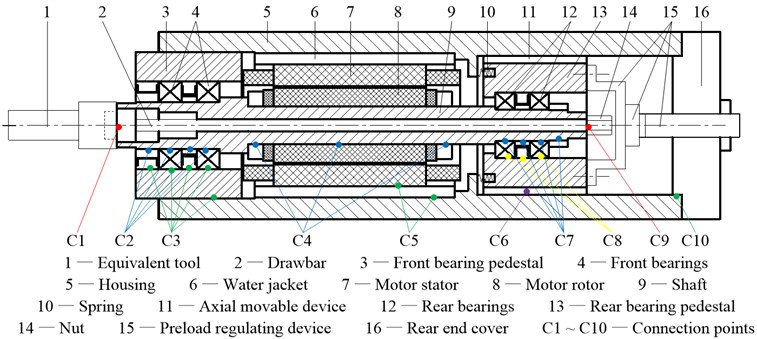
The schematic of the especially designed motorized spindle system is showed in Fig. 1. The shaft is supported by two pairs of angular contact ball bearings with double back-to-back arrangement. The front bearings and rear bearings are simultaneously preloaded by an adjustable preload mechanism, which includes a series of compressive springs, an axial movable rear bearing pedestal and a preload regulating device, to obtain the required preload for bearings and favorable dynamical properties for spindle. The bearings are individually cooled by oil/air lubrication. An asynchronous induction motor, adopting U/f control method, rated at 4.8 kW maximum power and up to 30000 rpm is located between the front and rear bearings. The motor stator is cooled by water. An equivalent tool is designed and mounted on the shaft by a standard HSK25C tool-holder interface and preloaded by a drawbar and a nut. The outside surface of the housing is designed to be a smooth cylindrical shape and easily fixed on the workbench.
Fig. 1Schematic of the especially designed motorized spindle system
2.1. Dynamical model for each rotor
In Fig. 1, it is obvious that there are three rotors in the motorized spindle system, the equivalent tool and drawbar, shaft and housing. And using the Timoshenko beam theory and FE theory [7], the three rotors can be modeled in the same way that the motion of each FE node of the rotors is described by three translational (, , ) and two rotational (, ) degrees of freedom:
And the equation of motion for each rotor is expressed by including the centrifugal force and gyroscopic effects as:
where , and are the rotor mass, rotor gyroscopic and rotor stiffness matrices respectively, ωr is the rotor speed, is the rotor mass matrix for the centrifugal force effect, is the rotor displacement vector, is the rotor external force vector.
2.2. Bearing stiffness matrix
The bearings support the shaft in the axial (), radial (, ) and angular (, ) directions and the state of preload has a great influence on the bearing support stiffness. The bearing model in this paper is adopted from [5] and the bearing stiffness matrix can be obtained by solving the balance equations of the balls and inner ring.
2.3. Dynamical model for system
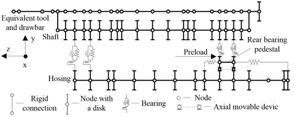
The three rotors are connected into a whole system by different methods. The equivalent tool and drawbar are mounted on the shaft by a tool-holder interface and a nut. At the connection points C1 and C9, they are consolidated together and it can be assumed that they have the same degrees of freedom, which is called the rigid connection. The machine parts mounted on the shaft and housing (bearing inner rings and motor rotor on the shaft at C2, C4 and C7, front bearing pedestal, motor stator and rear end cover on the housing at C3, C5 and C10 etc.) are assumed that they have the same degrees of freedom with those nodes, which are modeled as rigid disks with gyroscopic moment considered, using the method of being the same inertia with themselves. And it is called the node with a disk. The connection situation at C8 is same with that at C3 that the outer rings of bearings and bearing pedestals have the same degrees of freedom. However, at the connection point C6, the situation is not same with that at C3 that the rear bearing pedestal and housing have the same translational (, ) and rotational (, ) degrees of freedom but not the translational () degree of freedom because of the axial movable rear bearing pedestal and they are connected by the springs in the axial () direction. The shaft and pedestals are connected by bearings, which are simplified as nonlinear springs. Therefore, the system is modeled as a FE dynamical model, which is showed in Fig. 2. Then, assembling the equations of rotors and bearings and considering the effect of system damping, the equilibrium equation for the motorized spindle system is obtained:
where , , and are the mass, damping, gyroscopic and stiffness matrices of system respectively, is the system speed (when is not zero, the system is in the working state), is the system mass matrix for the centrifugal force effect, is the system displacement vector, is the system external force vector.
When the motorized spindle is in the non-working state ( is zero), the equilibrium equation of system is:
Fig. 2Dynamical model of system
2.4. Adjustable preload mechanism
The adjustable preload mechanism is showed in Fig. 3. The springs set at the end face of the rear bearing pedestal support it in the axial () direction with a constant force . The preload regulating device includes a piezoelectric stack force actuator for providing the adjustable force , a force sensor for measuring and a holder for connecting the force actuator and sensor to the rear bearing pedestal. The force, happened between the bearing outer rings and pedestals in the axial direction, is the preload . The three forces, , and , have an equilibrium relationship and it can be expressed as:
Fig. 3Adjustable preload mechanism of system
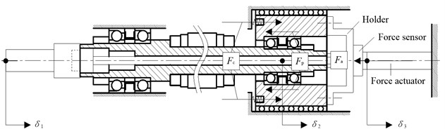
Under the function of the three forces, the tip of the equivalent tool and front bearing inner rings have a same axial displacement , the rear bearing inner rings have the axial displacements and the rear bearing pedestal has the axial displacements . It is obvious that there is a relationship between and :
where is the axial deformation of the rotors between the front and rear bearings caused by the thermal expansion and . Assuming the axial stiffness of front bearings and rear bearings is and respectively, the relationship can be obtained by:
The adjustable force from the piezoelectric stack force actuator is expressed by [13]:
where is the stiffness of the force actuator, is the piezoelectric coefficient and is the supply voltage. According to Eq. (5) and Eq. (8), we can adjust the preload by changing the supply voltage . And and can be obtained at the same time.
3. Experimental set-up
3.1. Experimental set-up in the non-working state
In order to obtain the dynamical properties of a motorize spindle system under different preload, an impact experiment under free-free boundary conditions has always been needed [14]. Since the vibration of the tool has a direct effect on the machining quality, it is of great necessity to study the transmission characteristics from other parts to the tool tip. The experimental set-up for FRF analysis is showed in Fig. 4, which consists of the especially designed motorized spindle system with an adjustable preload mechanism, a voltage source for supplying voltage for the piezoelectric stack force actuator, a hammer with a force sensor, a charge amplifier, an acceleration sensor, a displacement sensor and corresponding transmitters, a data acquisition system, a computer and corresponding software. The signals of with different can be measured directly to analyze the preload state of bearings. The signals of impact force from the hammer to the housing at #1, #2 and #3 can be measured and transmitted to the LMS data acquisition system through the charge amplifier. An acceleration sensor, mounted on the tip of the equivalent tool, can measure the vibration acceleration response signals which are transmitted to the same data acquisition system to obtain the FRFs of the system.
Fig. 4Experimental set-up in the non-working state
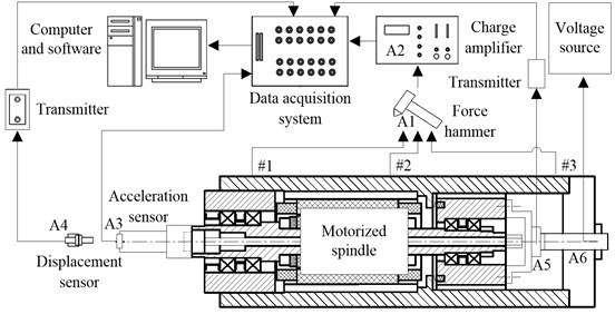
Fig. 5Experimental set-up in the working state
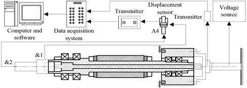
3.2. Experimental set-up in the working state
In the working state, the housing is fixed on the workbench and a lot of factors will generate the vibration of the equivalent tool, drawbar, shaft and rear bearing pedestal. Under different preload, the dynamical properties of the system can be obtained by measuring the radial and axial vibration states of the rotational equivalent tool and shaft. The experimental set-up for this study is showed in Fig. 5, which consists of the same motorized spindle system, voltage source, displacement sensors and transmitters, data acquisition system, computer and corresponding software as that in the non-working state. The signals of vibration displacement of the equivalent tool and shaft at &1, and &2 can be measured by the displacement sensors and transmitted to the LMS data acquisition system through the corresponding transmitters for analyzing the dynamical properties of the system.
3.3. Experimental apparatus
The electronic equipments used in the experimental set-up are numbered A1 to A6 and their parameters are listed in Table 1. The parameters of the angular contact ball bearings used in the spindle system are listed in Table 2.
Table 1Parameters of the electronic equipments
No. | Type | Measurement range | Sensitivity | Nonlinear error |
A1 | CL-YD-303 | 0-2000N | 3.650 pC/N | 1 % |
A2 | YE5850 | –10-10 V | 100 mV/N | 1 % |
A3 | PCB 356A32 | –500-500 m·s-2 | -10.38 mV/m·s-2 -10.27 mV/m·s-2 -10.11 mV/m·s-2 | 0.5 % |
A4 | WD501 | 0-1 mm | 0.1 μm/mV | 1 % |
A5 | XL-7SW | 0-1000 N | 50 mV/N | 1 % |
A6 | PT150 | 0-20 μm 0-5000 N | 250 N/μm 0.125 μm/V | 1 % |
Table 2Parameters of the bearings
Parameters | Front bearing (F) | Rear bearing (R) |
Type | B7005CD/P4A | B7003CD/P4A |
Material | Steel | Steel |
Ball diameter (mm) | 5.5 | 4 |
Number of balls | 15 | 13 |
Inner groove curvature | 0.57 | 0.57 |
Outer groove curvature | 0.54 | 0.54 |
Inner raceway diameter (mm) | 30.480 | 21.985 |
Outer raceway diameter (mm) | 41.520 | 30.015 |
4. Validations and analysis
For the dynamical properties analysis of this especially designed spindle system with an adjustable preload mechanism, some computer programs have been developed by Newton-Raphson iteration method to calculate the bearings nonlinear stiffness and the system equilibrium equation in the non-working state, and subspace iteration method to obtain the inherent characteristics of the FE dynamical model in the working state.
4.1. Bearing stiffness analysis
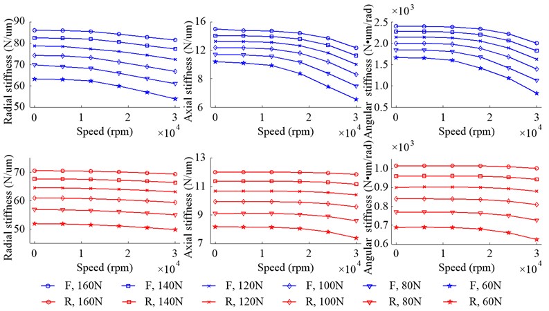
Both of the front bearing and rear bearing are analyzed in this paper and the bearing stiffness is showed in Fig. 6. It is obvious that the radial stiffness, axial stiffness and angular stiffness decrease with the speed rising because of the effects of the centrifugal force and gyroscopic moment of the ball and this phenomenon was called softening of bearing [5]. When at a lower speed, the centrifugal force and gyroscopic moment are very small, so the bearing stiffness almost keeps constant. However, when the speed exceeds 11000 rpm, the bearing stiffness is gradually softened since the value of centrifugal force and gyroscopic moment increases rapidly. With the increasing of , the contact between balls and rings of bearing is closer, so the bearing stiffness rises. And the radial, axial and angular stiffness of front bearing, when 160 N and speed is 12000 rpm, increases by 36.40 %, 44.87 % and 44.62 % over that 60 N, respectively, and the same data of rear bearing are 36.08 %, 47.18 % and 42.69 %. It also can be observed that the increase of reduces the downward trend of bearing stiffness. Compared with the front bearing, the stiffness of rear bearing is smaller and its downward trend is slower.
Fig. 6Stiffness of bearings with different Fp due to the change of speed
4.2. Validations and analysis for axial displacement in the non-working state
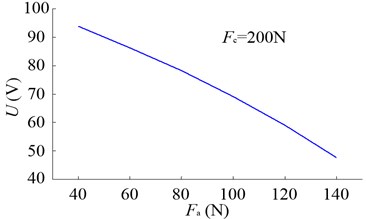
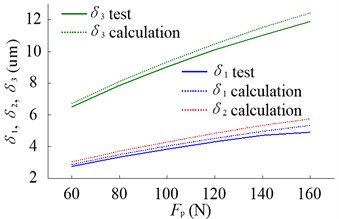
When changing the supply voltage , the preload can be adjusted, and Fig. 7 shows the tested and calculated results of , , , , and in the non-working state. According to Eq. (5), if reducing the adjustable force , will be enlarged, and the supply voltage should be turned up accordingly. With the increasing of , , and rise. The axial displacement of rear bearing inner rings () is a little bigger than that of front bearing inner rings () because of the axial elastic deformation of spindle (). The axial displacement of rear bearing pedestal () is approximately twice as large as the axial displacement of equivalent tool (), which is mainly caused by the relative axial displacement of the inner and outer rings of rear bearing (-).
Fig. 7a) Relationship between Fa and U, b) effects of Fp on δ1, δ2 and δ3
a)
b)
4.3. Inherent characteristics analysis and validation in the non-working state
The inherent modes of the system, in the non-working state, include radial vibration and axial vibration.
4.3.1. Inherent modal shapes
Fig. 8Inherent modal shapes of radial vibration in the non-working state when Fp= 100 N
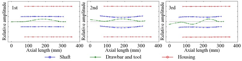
Fig. 9Inherent modal shapes of axial vibration in the non-working state when Fp= 100 N
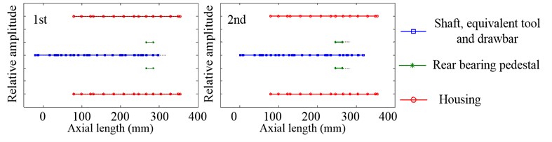
Since the inherent modal shapes of system with different preload are almost no change, there is the analysis of inherent modal shape only when 100 N. Fig. 8 shows the first three inherent modal shapes of the radial vibration. The first is the vibration of the drawbar, which has one vibration wave, with little relative vibration amplitude on the shaft. The second is the vibration of the equivalent tool, drawbar and shaft, and the equivalent tool and drawbar have two vibration waves while the shaft has only one. The third is also the vibration of the equivalent tool, drawbar and shaft, like the second, while the equivalent tool and drawbar have three vibration waves and the shaft has two. Fig. 9 shows the first two inherent modal shapes of the axial vibration. And both of them are the rigid body vibration happened on the shaft, equivalent tool, drawbar and rear bearing pedestal. The first is the axial vibration of the shaft, equivalent tool and drawbar while the relative vibration amplitude of the rear bearing pedestal is nearly zero. Compared with the first inherent modal shape of axial vibration, the second is just the opposite. In all of the inherent modal shapes of radial and axial vibration, the housing has little relative vibration amplitude.
4.3.2. Test
The tests have been done under different while the results under 100 N are analyzed in this part only. The modal damping ratios obtained from these tests are listed in Table 3 and used for the simulations.
Fig. 10 shows the tested and calculated FRFs of radial vibration at the equivalent tool tip. Within 0-1500 Hz frequency range, there are three amplitude peaks which correspond to the three inherent modal shapes of radial vibration. Theoretically, the radial FRFs in -direction and -direction are absolutely identical. However, the tested data has some differences between -direction and -direction because of the unsymmetrical structure of the experimental set-up. When at #1 and #2, the overall trends of tested and calculated FRFs are close and the maximum peak happens at the second order inherent frequency, and because the relative amplitude of the first inherent modal shape at the tool tip is nearly zero, which is showed in Fig. 8, the peak at the first order inherent frequency is so small. Compared to #1, the amplitude of FRFs at #2 is bigger, which indicates the impact from middle part of the housing can cause the vibration of the tool more easily. When at #3, the amplitude of FRFs are smaller than that at #1 and #2, so the impact from the hind part of housing can cause the vibration of the tool more difficult. And the overall trends of tested and calculated FRFs, at #3, are a little different and the possible reason for this phenomenon is that the proposed model is not so perfect that can predict all the dynamical properties of the radial vibration.
Table 3Tested damping ratios when Fp= 100 N
#1 | #2 | #3 | |||||||
First mode | 0.87 % | 0.93 % | 1.05 % | 0.89 % | 0.74 % | 1.06 % | 0.63 % | 0.64 % | 1.02 % |
Second mode | 0.43 % | 0.38 % | 1.22 % | 0.45 % | 0.57 % | 1.48 % | 0.57 % | 0.52 % | 1.73 % |
Third mode | 0.58 % | 0.54 % | – | 0.32 % | 0.39 % | – | 0.39 % | 0.43 % | – |
Fig. 10Tested and calculated FRFs of radial vibration at the equivalent tool tip, impact from #1, #2 and #3 when Fp= 100 N
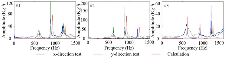
Fig. 11The tested and calculated FRFs of axial vibration at the equivalent tool tip, impact from #1, #2 and #3 when Fp= 100 N
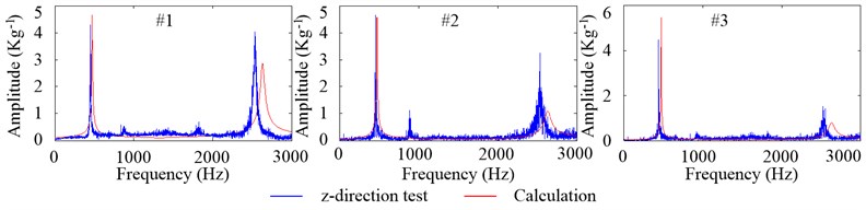
Fig. 11 shows the tested and calculated FRFs of axial vibration at the equivalent tool tip. Within 0-3000 Hz frequency range, there are two amplitude peaks which correspond to the two inherent modal shapes of axial vibration. At all of the impact points, the overall trends of tested and calculated FRFs are close and the maximum peak happens at the first order inherent frequency. From #1 to #3, the amplitudes of FRFs at the first order inherent frequency are almost no change while the amplitudes at the second order inherent frequency reduce. And this phenomenon indicates that the impacts, from the front part to the hind part of the housing, have the identical and weakening effects on the first and second inherent modal shapes of axial vibration of the tool, respectively.
4.3.3. Inherent frequencies
Fig. 12 shows the first three inherent frequencies of radial vibration. The inherent frequencies in different direction, at the same impact point, have slight differences due to the unsymmetrical structure of system as mentioned above. Since the first inherent modal shape has little relation with bearing radial stiffness, which increases with the increasing of , the enlargement of has a little effect on the first inherent frequencies. While the second and third inherent frequencies rise rapidly with the increasing of because of the strong correlation between the bearing radial stiffness and their corresponding inherent modal shapes. It is obvious that, compared with the first and second inherent frequencies, the error between the calculated results and tested data at the third is larger. Fig. 13 shows the first two inherent frequencies of axial vibration. The first two inherent modal shapes of axial vibration have strong correlation with the bearing axial stiffness, with the increasing of which rises rapidly. And compared with at the first inherent frequency, the calculation error at the second is bigger.
Fig. 12Inherent frequencies of radial vibration in the non-working state due to the change of Fp
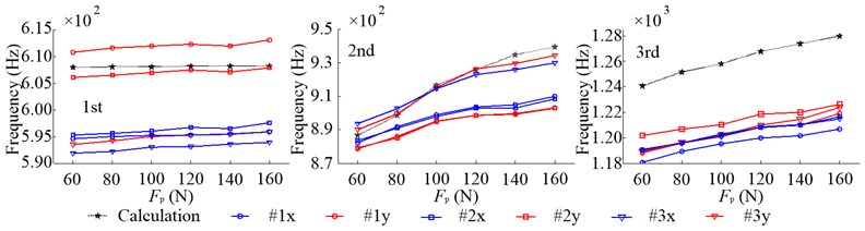
Fig. 13Inherent frequencies of axial vibration in the non-working state due to the change of Fp
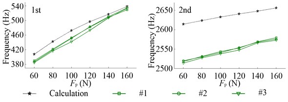
Fig. 14Variation domains of inherent frequencies in the non-working state due to the change of Fp from 60 N to 160 N
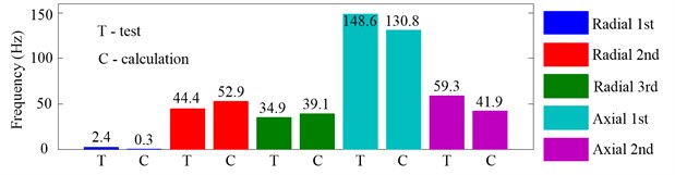
Fig. 14 shows the variation domains of inherent frequencies in the non-working state due to the change of from 60 N to 160 N. It is obvious that the first inherent frequencies of axial vibration are most affected by the increasing of and their variation domains are up to 148.6 Hz (test) and 130.8 Hz (calculation). The second inherent frequencies of the radial and axial vibration take the second place, the variation domains of which are about 50 Hz. The first inherent frequencies of radial vibration are the least affected.
4.4. Validations and analysis for axial displacement in the working state
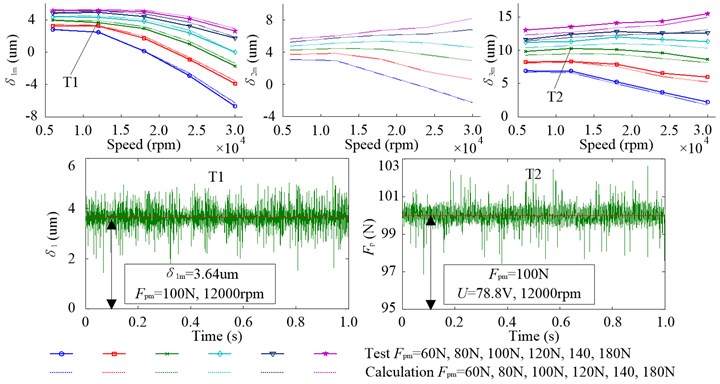
When the motorized spindle is in the working state, the axial displacements , , and preload are not constants any more. Therefore, the preload state can be studied by analyzing the mean of , , and (, , and ). Fig. 15 shows , , and two tested points T1 and T2 at 12000 rpm, 100 N, 78.8 V in 1 second. With the increasing of , , , and gradually rise and this variation trend is identical to that in the non-working state. However, with the increasing of speed shows the downward trend, the reason for which is that the rising speed increases the centrifugal force of front bearing ball and makes its inner ring move toward the negative direction of . Due to the effects of the centrifugal force of rear bearing ball (the value of - increases) and thermal expansion of spindle ( increases), and decrease under low and increase under high .
Fig. 15Mean of the axial displacement δ1, δ2 and δ3 and test curves of T1 and T2 in 1 second
4.5. Inherent characteristics analysis and validation in the working state
In the working state, the housing is fixed on the workbench, so the dynamical model of system only takes the shaft, rear bearing pedestal, drawbar and equivalent tool into account. The same as in the non-working state, the inherent modes of the system in the working state also include radial vibration and axial vibration.
4.5.1. Inherent modal shapes
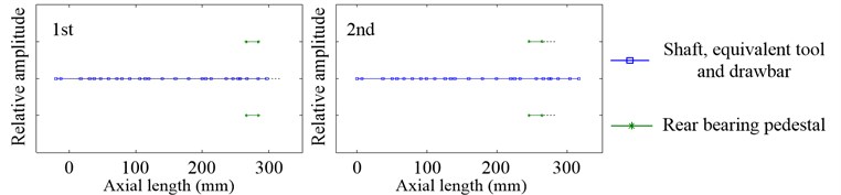
Since the speed and preload have little effect on the inherent modal shapes of system, there is the analysis of it only when 12000 rpm and 100 N. Fig. 16 and Fig. 17 show the first three inherent modal shapes of the radial vibration and first two inherent modal shapes of the axial vibration, respectively. It can be easily found that the vibration state of the shaft, equivalent tool and drawbar of all the inherent modal shapes in the working state are very close to that in the non-working state. And this is because the inherent modal shape of housing has little relative vibration amplitude in the non-working state and little effect on the vibration of the shaft, equivalent tool and drawbar.
Fig. 16Inherent modal shapes of radial vibration in the working state when12000 rpm and Fpm= 100 N
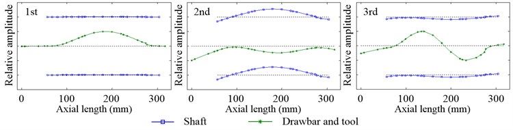
Fig. 17Inherent modal shapes of axial vibration in the working state when 12000 rpm and Fpm= 100 N
4.5.2. Test
The tests have been done under different and speed while only the results at 12000 rpm are analyzed in this part.
Fig. 18 shows the radial vibration displacement spectrums at &1 with different . There are three amplitude peaks in the frequency range of 580 Hz to 620 Hz, 850 Hz to 930 Hz and 1140 Hz to 1240 Hz, respectively, which correspond to the three inherent modal shapes of radial vibration. Since the relative vibration amplitude of the first inherent modal shape at &1 is very small, the amplitude peaks at the first inherent frequency are little and just less than 0.3 μm. The amplitude peaks at the second and third inherent frequencies are about 1.5 μm and 0.8 μm, respectively. With the increasing of , the amplitude peaks at the first inherent frequency are much more intensive than those at the second and third inherent frequencies, and this phenomenon indicates that the preload has little effect on the first inherent frequency while a great influence on the second and third inherent frequencies.
Fig. 18Radial vibration displacement spectrums at &1 with different Fpm when 12000 rpm
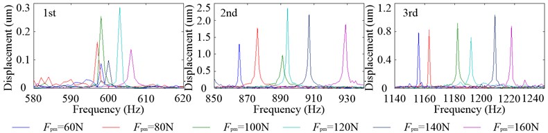
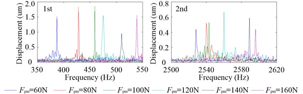
Fig. 19 shows the axial vibration displacement spectrums at &2 with different . There are two amplitude peaks in the frequency range of 350 Hz to 550 Hz and 2500 Hz to 2620 Hz, respectively, which correspond to the two inherent modal shapes of axial vibration. The amplitude peaks at the first and second inherent frequencies are about 1.5 μm and 0.5 μm, respectively, which indicates that the first inherent mode happens more easily. The preload has a great influence on the first two inherent frequencies, so with the increasing of the amplitude peaks at both of them are dispersive.
Fig. 19Axial vibration displacement spectrums at &2 with different Fpm when 12000 rpm
4.5.3. Inherent frequencies
Fig. 20 shows the first three inherent frequencies of radial vibration. The calculated inherent frequency of radial vibration of the high speed rotor has two branches (forward and backward) affected by the centrifugal force and gyroscopic moment [6], while in this part only the backward branch is analyzed. At low speed, for example at 6000 rpm, the inherent frequencies are a little bigger than that at 0 rpm (in the non-working state). And the reason for it is that when the housing is fixed on the workbench the stiffness of rotors system will increase and the corresponding inherent frequencies also rise. Because of the effect of centrifugal force, gyroscopic moment and decline of bearing radial stiffness, with the increasing of speed, all of the first three inherent frequencies decrease. Due to the same reason as in the non-working state, the enlargement of has a little effect on the first inherent frequencies while a strong effect on the second and third inherent frequencies. Fig. 21 shows the first two inherent frequencies of axial vibration. Due to the same reason for the radial vibration, the inherent frequencies of axial vibration, at low speed, are a little bigger than that at 0 rpm. Because of the decline of bearing axial stiffness, with the increasing of speed, both of the first two inherent frequencies decrease. While, with the increasing of , they rise and show the same variation trend as the bearing axial stiffness.
Fig. 20Inherent frequencies of radial vibration in the working state with different Fpm due to the change of speed
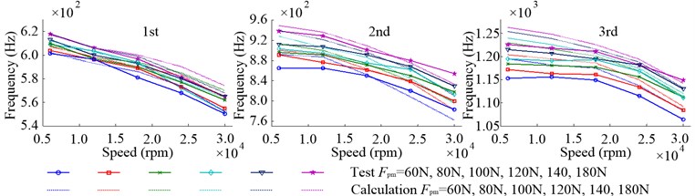
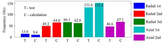
Fig. 22 shows the variation domains of inherent frequencies in the working state due to the change of from 60 N to 160 N when 12000 rpm. Like in the non-working state, the first inherent frequencies of axial vibration are most affected by the increasing of and their variation domains are up to 131.6 Hz (test) and 152.4 Hz (calculation). The second and third of radial vibration and second of axial vibration take the second place, the variation domains of which are about 60 Hz. However, the effect of on the first inherent frequencies of radial vibration is more obvious than that in the non-working state and the variation domains of which are up to 13.6 Hz (test) and 9.6 Hz (calculation).
Fig. 21Inherent frequencies of axial vibration in the working state with different Fpm due to the change of speed
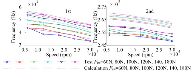
Fig. 22Variation domains of inherent frequencies in the working state due to the change of Fpm from 60 N to 160 N when 12000 rpm
4.6. Effect of on the spindle stiffness and machining stability
Fig. 23 shows the spindle stiffness at the equivalent tool tip. With the increasing of speed, the radial and axial stiffness decrease and the downward trend is consistent with the stiffness of front bearing. The radial stiffness of spindle at the equivalent tool tip is about 60 % to 70 % of the radial stiffness of front bearing and the axial stiffness of spindle is equal to the axial stiffness of front bearing. It is obvious that the increase of raises both of the radial and axial stiffness of spindle.
Fig. 23Spindle stiffness at the equivalent tool tip due to the change of speed
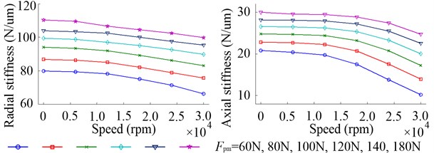
Fig. 24a) Predicted stability lobes without speed effect when Fpm= 100 N, b) bmax due to the change of Fpm
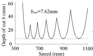
a)
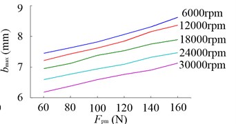
b)
The chatter stability lobes at the equivalent tool tip of the especially designed motorized spindle, used for face milling, are predicted. The analytical chatter prediction theory of Altintas and Budak [14] is used and the results are showed in Fig. 24. The depth of cut without speed effect when 100 N has a maximum value 7.62 mm. When considering the speed effect, the decline of spindle radial stiffness makes the decrease. While with the increasing of , the spindle radial stiffness makes the spindle obtain higher stability. At 12000 rpm, compared with under 60 N, under 160 N increases by 15.95 %.
5. Conclusions
In this paper, a FE model for dynamical analysis of the especially designed motorized spindle with an adjustable preload mechanism is developed and validated experimentally in both of the non-working and working states to predict the dynamical properties of spindle system under different preload. According to the results, the following conclusions are obtained:
a) The speed and preload have a small effect on the inherent modal shapes of system. The inherent modal shapes of the shaft, drawbar, tool and rear bearing pedestal in both of the non-working and working state are identical. And the inherent modal shapes of radial and axial vibration are elastic body vibration and rigid body vibration, respectively.
b) The inherent frequencies in both of the non-working and working states are close because of the identical inherent modal shapes. Unlike the inherent modal shapes, the inherent frequencies are seriously affected by the speed and preload. The softening effect of bearing stiffness, with the increasing of speed, makes the inherent frequencies of system reduce. While the higher preload increases the inherent frequencies and first inherent frequency of axial vibration has most obvious performance.
c) The spindle stiffness largely depends on the stiffness of front bearing, which is increased by the rising of preload. And the same variation trend happens on the chatter stability of system.
d) In order to obtain perfect dynamical properties of a motorized spindle system, which include the low vibration amplitude, high limit speed (inherent frequencies), high spindle stiffness, high chatter stability and so on, we can choose a suitable preload. However, the large amount of bearing heat generation caused by high bearing preload should be considered at the same time [16-17].
References
-
Abele E., Altintas Y., Brecher C. Machine tool spindle units. CIRP Annals-Manufacturing Technology, Vol. 59, Issue 2, 2010, p. 1-22.
-
Terman T., Bollinger J. G. Graphical method for finding optimum bearing span for overhung shafts. Journal of Machine Design, Vol. 37, Issue 12, 1965, p. 159-162.
-
Sharan A. M., Sankar S., Sankar T. S. Dynamic analysis and optimal selection of parameters of a finite-element modeled lathe spindle under random cutting forces. Journal of Vibration Acoustics Stress and Reliability in Design, Vol. 105, Issue 4, 1983, p. 467-475.
-
Jones A. A general theory for elastically constrained ball and radial roller bearings under arbitrary load and speed conditions. Journal of Basic Engineering, Vol. 82, Issue 2, 1960, p. 309-320.
-
Li S. S., Chen X. Y., Zhang G., Wang C. L., Yang L. X., Chen C. J. Analysis of dynamic supporting stiffness about spindle bearings at extra high-speed in electric spindles. Chinese Journal of Mechanical Engineering, Vol. 42, Issue 11, 2006, p. 60-65.
-
Han S. M., Benaroya H., Wei T. Dynamics of transversely vibrating beams using four engineering theories. Journal of Sound and Vibration, Vol. 225, Issue 5, 1999, p. 935-988.
-
Nelson H. D. A finite rotation shaft element using Timoshenko beam theory. Journal of Mechanical Design, Vol. 102, 1980, p. 793-803.
-
Li H. Q., Shin Y. C. Integrated dynamic thermo-mechanical modeling of high speed spindles, Part 1: Model development. Journal of Manufacturing Science and Engineering, Vol. 126, Issue 1, 2004, p. 148-158.
-
Li H. Q., Shin Y. C. Integrated dynamic thermo-mechanical modeling of high speed spindles, Part 2: Solution procedure and validations. Journal of Manufacturing Science and Engineering, Vol. 126, Issue 1, 2004, p. 159-168.
-
Chen X. A., Liu J. F., He Y., Zhang P., Shan W. T. An integrated model for high-speed motorized spindles – dynamic behaviors. Proceedings of the Institution of Mechanical Engineers, Part C-Journal of Mechanical Engineering Science, Vol. 227, Issue 11, 2013, p. 2467-2478.
-
Cao H. R., Holkup T., Altintas Y. A comparative study on the dynamics of high speed spindles with respect to different preload mechanisms. International Journal of Advanced Manufacture Technology, Vol. 57, Issue 9-12, 2011, p. 871-883.
-
Chen J. S., Chen K. W. Bearing load analysis and control of a motorized high speed spindle. International Journal of Machine Tools & Manufacture, Vol. 45, Issue 12-13, 2007, p. 1487-1493.
-
Palazzolo A. B., Lin R. R., Alexander R. M., Kascak A. F., Montague J. Piezoelectric pushers for active vibration control of rotating machinery. Journal of Vibration Acoustics Stress and Reliability in Design, Vol. 11, Issue 3, 1989, p. 298-305.
-
Forestier F., Gagnol V., Ray P. Model-based cutting prediction for a self-vibratory drilling head-spindle system. International Journal of Machine Tools & Manufacture, Vol. 52, Issue 1, 2012, p. 59-68.
-
Altintas Y., Budak E. Analytical prediction of stability lobes in milling. CIRP Annals Manufacturing Technology, Vol. 44, Issue 1, 1995, p. 357-362.
-
Bossmanns B., Tu J. F. A thermal model for high speed motorized spindles. International Journal of Machine Tools & Manufacture, Vol. 39, Issue 9, 1999, p. 1345-1366.
-
Bossmanns B., Tu J. F. A power flow model for high speed motorized spindles – heat generation characterization. Journal of Manufacturing Science and Engineering, Vol. 123, Issue 3, 2001, p. 494-505.
About this article
This work is financially supported by National Natural Science Foundation of China (No. 51005259).
